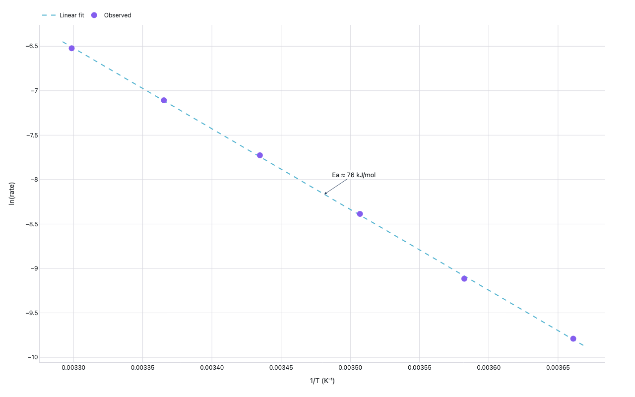
Arrhenius plot

Python Code

"""Chemical Kinetics — Arrhenius plot (Hecht-Conrad 1889 data)."""
from pathlib import Path

# ── Palette + theme (matching the Plotly Studio gallery these charts ship in) ──
VIOLET, TEAL, GREEN, PINK, ORANGE = "#845EEE", "#52B3D0", "#55B685", "#DA5597", "#E9A23B"
PRIMARY, SECONDARY = VIOLET, TEAL
COLORWAY = [VIOLET, TEAL, GREEN, PINK, ORANGE]
BG, TEXT, GRID, MUTED = "#ffffff", "#1c2024", "#d9d9e0", "#60646c"
FONT = "Inter, -apple-system, BlinkMacSystemFont, sans-serif"
COLORSCALE = [[0, "rgba(132, 94, 238, 0.05)"], [1, "rgba(132, 94, 238, 0.9)"]]


def apply_theme(fig):
    """Light gallery theme: white background, Inter font, soft gridlines."""
    fig.update_layout(
        paper_bgcolor=BG, plot_bgcolor=BG, colorway=COLORWAY,
        font=dict(family=FONT, color=TEXT, size=12),
        legend=dict(font=dict(color=TEXT)),
        hoverlabel=dict(bgcolor="#f0f0f3", font=dict(color=TEXT, family=FONT), bordercolor=GRID),
    )
    fig.update_xaxes(gridcolor=GRID, linecolor=GRID, zerolinecolor=GRID)
    fig.update_yaxes(gridcolor=GRID, linecolor=GRID, zerolinecolor=GRID)


def fetch_csv(url, **kwargs):
    import io
    import pandas as pd
    import requests
    r = requests.get(url, timeout=60)
    r.raise_for_status()
    return pd.read_csv(io.StringIO(r.text), **kwargs)


def fetch_json(url):
    import requests
    r = requests.get(url, timeout=60)
    r.raise_for_status()
    return r.json()

import numpy as np
import plotly.graph_objects as go


# Hecht-Conrad 1889: ethoxide + methyl iodide reaction rates
T_C = [0, 6, 12, 18, 24, 30]       # Celsius
RATE = [5.60e-5, 11.0e-5, 22.8e-5, 44.1e-5, 81.9e-5, 147.0e-5]  # relative rate


def generate():
    T_K = np.array([t + 273.15 for t in T_C])
    inv_T = 1.0 / T_K
    ln_rate = np.log(RATE)

    # Linear fit: ln(k) = -Ea/R * (1/T) + ln(A)
    slope, intercept = np.polyfit(inv_T, ln_rate, 1)
    R = 8.314  # J/(mol·K)
    Ea = -slope * R / 1000.0  # kJ/mol

    print(f"  slope = {slope:.1f}  intercept = {intercept:.3f}")
    print(f"  Ea ≈ {Ea:.1f} kJ/mol")

    x_fit = np.linspace(inv_T.min() * 0.998, inv_T.max() * 1.002, 200)
    y_fit = slope * x_fit + intercept

    fig = go.Figure()

    # Fitted line
    fig.add_trace(go.Scatter(
        x=x_fit,
        y=y_fit,
        mode="lines",
        name="Linear fit",
        line=dict(color=TEAL, width=2, dash="dash"),
        hoverinfo="skip",
    ))

    # Data points
    fig.add_trace(go.Scatter(
        x=inv_T,
        y=ln_rate,
        mode="markers",
        name="Observed",
        marker=dict(size=12, color=VIOLET, symbol="circle"),
        customdata=list(zip(T_C, RATE)),
        hovertemplate=(
            "T = %{customdata[0]}°C<br>"
            "1/T = %{x:.5f} K⁻¹<br>"
            "ln(rate) = %{y:.3f}<extra></extra>"
        ),
    ))

    # Annotation for Ea
    mid_idx = len(x_fit) // 2
    fig.update_layout(
        xaxis=dict(
            title="1/T (K⁻¹)",
            tickformat=".5f",
        ),
        yaxis=dict(title="ln(rate)"),
        legend=dict(orientation="h", y=1.05, x=0),
        annotations=[dict(
            x=x_fit[mid_idx],
            y=y_fit[mid_idx],
            text=f"Ea ≈ {Ea:.0f} kJ/mol",
            showarrow=True,
            arrowhead=2,
            ax=60,
            ay=-40,
            font=dict(size=13),
            bgcolor="rgba(255,255,255,0.85)",
        )],
        margin=dict(t=50, b=70, l=80, r=60),
    )
    apply_theme(fig)
    return fig


fig = generate()
fig.show()

Made with Plotly