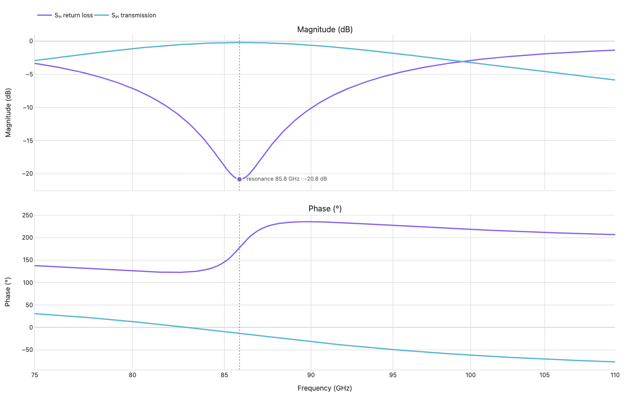
Bode plot

Python Code

"""Bode plot — measured coplanar-waveguide ring-slot antenna (VNA, W-band)."""


import numpy as np
import plotly.graph_objects as go
from plotly.subplots import make_subplots
import requests, warnings


# Real vector-network-analyzer sweep of a CPW ring-slot antenna, 75–110 GHz
# (W-band), shipped as example data with scikit-rf. Touchstone .s2p, real/imag
# S-parameters referenced to 50 Ω. S11 = return loss (how well the antenna is
# matched), S21 = transmission through the two-port fixture.
URL = "https://raw.githubusercontent.com/scikit-rf/scikit-rf/master/skrf/data/ring%20slot.s2p"


def generate():
    print("fetching measured ring-slot antenna S-parameters (scikit-rf) …")
    warnings.filterwarnings("ignore")
    requests.packages.urllib3.disable_warnings()
    r = requests.get(URL, verify=False, timeout=30)
    r.raise_for_status()

    # Touchstone: skip '!' comments and the '#' option line; data rows start
    # with a digit. Columns: freq ReS11 ImS11 ReS21 ImS21 ReS12 ImS12 ReS22 ImS22
    rows = [ln.split() for ln in r.text.splitlines() if ln[:1].isdigit()]
    a = np.array(rows, dtype=float)
    f = a[:, 0]  # frequency, GHz (header declares "# GHz")
    print(f"  parsed {len(f)} frequency points, {f[0]:.0f}–{f[-1]:.0f} GHz")

    def db_phase(re, im):
        z = re + 1j * im
        mag = 20 * np.log10(np.abs(z))
        ph = np.unwrap(np.angle(z)) * 180 / np.pi
        return mag, ph

    s11_db, s11_ph = db_phase(a[:, 1], a[:, 2])
    s21_db, s21_ph = db_phase(a[:, 3], a[:, 4])

    # Resonance: deepest return loss (best match) — where the antenna radiates.
    res_i = int(np.argmin(s11_db))
    res_f, res_db = f[res_i], s11_db[res_i]

    fig = make_subplots(
        rows=2, cols=1, shared_xaxes=True, vertical_spacing=0.07,
        subplot_titles=("Magnitude (dB)", "Phase (°)"),
    )

    traces = [
        ("S₁₁ return loss", VIOLET, s11_db, s11_ph),
        ("S₂₁ transmission  ", TEAL, s21_db, s21_ph),
    ]
    for name, color, mag, ph in traces:
        fig.add_trace(go.Scatter(
            x=f, y=mag, mode="lines", name=name,
            line=dict(color=color, width=2.5), legendgroup=name,
            hovertemplate="%{x:.2f} GHz<br>%{y:.2f} dB<extra></extra>",
        ), row=1, col=1)
        fig.add_trace(go.Scatter(
            x=f, y=ph, mode="lines", name=name,
            line=dict(color=color, width=2.5), legendgroup=name,
            showlegend=False,
            hovertemplate="%{x:.2f} GHz<br>%{y:.1f}°<extra></extra>",
        ), row=2, col=1)

    # Mark the return-loss resonance.
    fig.add_vline(x=res_f, line=dict(color=MUTED, width=1, dash="dot"), row=1, col=1)
    fig.add_vline(x=res_f, line=dict(color=MUTED, width=1, dash="dot"), row=2, col=1)
    fig.add_trace(go.Scatter(
        x=[res_f], y=[res_db], mode="markers+text",
        marker=dict(color=VIOLET, size=11, symbol="circle", line=dict(color="white", width=2)),
        text=[f"  resonance {res_f:.1f} GHz · {res_db:.1f} dB"],
        textposition="middle right", textfont=dict(color=MUTED, size=11),
        showlegend=False,
        hovertemplate=f"Resonance: {res_f:.1f} GHz, {res_db:.1f} dB<extra></extra>",
    ), row=1, col=1)

    fig.update_xaxes(type="log", row=1, col=1)
    fig.update_xaxes(type="log", title_text="Frequency (GHz)", row=2, col=1)
    fig.update_yaxes(title_text="Magnitude (dB)", row=1, col=1)
    fig.update_yaxes(title_text="Phase (°)", row=2, col=1)

    fig.update_layout(
        title=dict(text="Bode Plot — Measured Ring-Slot Antenna (VNA, W-band)", x=0.5),
        legend=dict(orientation="h", y=1.08),
        margin=dict(t=70, b=50, l=70, r=40),
        height=540,
    )
    return fig


if __name__ == "__main__":
    generate()

Made with Plotly