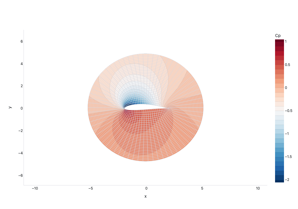
Carpet plot of an airfoil C-mesh with pressure-coefficient contours

Python Code

"""Aerospace — Carpet plot of an airfoil C-mesh with pressure-coefficient contours."""


import numpy as np
import plotly.graph_objects as go


URL = "https://raw.githubusercontent.com/bcdunbar/datasets/master/airfoil_data.json"


def generate():
    # The dataset is a 7-element list: data[0] holds the curvilinear mesh
    # (parametric a/b coordinates + their cartesian x/y positions) and
    # data[1] holds the pressure coefficient Cp sampled on that same mesh.
    # a/b/x/y/z are passed to the carpet traces as-is (a is 1D, the rest 2D
    # of shape len(b) x len(a)) — no flattening.
    try:
        raw = fetch_json(URL)
        mesh, field = raw[0], raw[1]
        a, b = mesh["a"], mesh["b"]
        x, y = mesh["x"], mesh["y"]
        z = field["z"]
        print(f"Loaded: a={len(a)}, b={len(b)}, mesh={len(x)}x{len(x[0])}")

    except Exception as e:
        print(f"Download failed ({e}), using synthetic O-mesh around a body")
        a = np.linspace(1.0, 5.0, 31)          # radial station (inner dim)
        b = np.linspace(0.0, 2 * np.pi, 71)     # angular station (outer dim)
        R, TH = np.meshgrid(a, b)               # (71, 31)
        x = (R * np.cos(TH)).tolist()
        y = (R * np.sin(TH)).tolist()
        z = (-2.0 / R * np.cos(TH) - 0.5).tolist()  # dipole-like pressure field
        a, b = a.tolist(), b.tolist()

    fig = go.Figure()

    # Carpet base: the deformed grid itself. a/b ticks are mesh indices, not
    # physically meaningful, so hide the labels and let the grid carry the eye.
    fig.add_trace(go.Carpet(
        a=a,
        b=b,
        x=x,
        y=y,
        aaxis=dict(showticklabels="none", gridcolor=GRID, startline=False, endline=False),
        baxis=dict(showticklabels="none", gridcolor=GRID, startline=False, endline=False),
        name="Mesh",
    ))

    # Pressure-coefficient contours filled onto the same carpet.
    # Clip the contour window to the physically interesting band: the
    # free stream sits near Cp=0 and the leading-edge suction peak dips to
    # roughly -6, which would otherwise wash the whole field into one color.
    fig.add_trace(go.Contourcarpet(
        a=a,
        b=b,
        z=z,
        colorscale="RdBu",
        reversescale=True,
        contours=dict(start=-2.0, end=1.0, size=0.1),
        line=dict(width=0.4, color="rgba(0,0,0,0.25)"),
        colorbar=dict(title="Cp"),
        name="Cp",
    ))

    fig.update_layout(
        xaxis=dict(title="x", showgrid=False, zeroline=False),
        yaxis=dict(title="y", showgrid=False, zeroline=False,
                   scaleanchor="x", scaleratio=1),
    )

    return fig


if __name__ == "__main__":
    generate()

Made with Plotly