CMB Power Spectrum

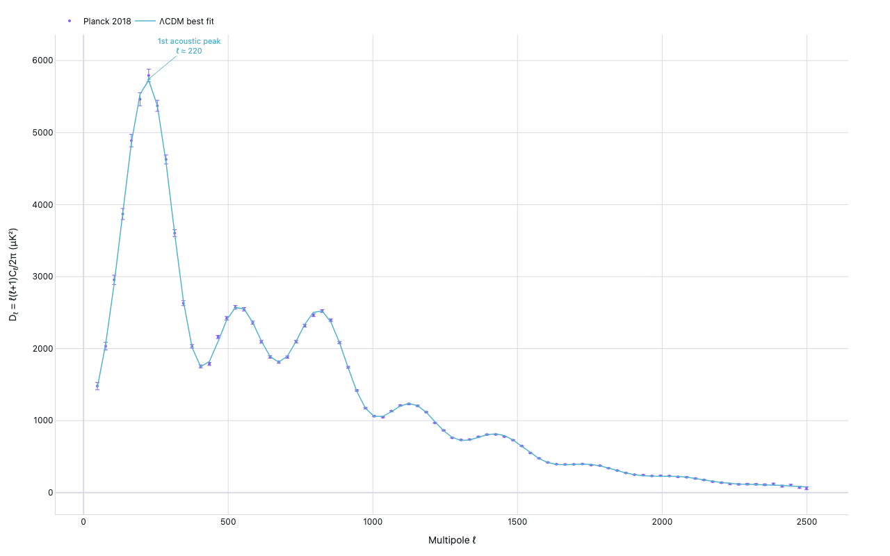
Python Code

"""Cosmology — CMB Power Spectrum (Planck 2018)."""


import io
import numpy as np
import pandas as pd
import requests
import plotly.graph_objects as go

URL = "http://pla.esac.esa.int/pla/aio/product-action?COSMOLOGY.FILE_ID=COM_PowerSpect_CMB-TT-binned_R3.01.txt"


def synthetic_cmb():
    """Generate a CMB-like TT power spectrum with three acoustic peaks."""
    ell = np.concatenate([
        np.arange(2, 30),
        np.arange(30, 100, 2),
        np.arange(100, 800, 4),
        np.arange(800, 2500, 10),
    ])
    # Approximate shape: Sachs-Wolfe plateau, acoustic peaks, damping
    # Peaks at ell ~ 220, 540, 810
    def cmb_approx(l):
        # SW plateau
        sw = 1000 * (l / 10) ** (-0.1) * np.exp(-((l / 2000) ** 2))
        # Acoustic peaks (three)
        p1 = 5500 * np.exp(-((l - 220) ** 2) / (2 * 60**2))
        p2 = 2500 * np.exp(-((l - 540) ** 2) / (2 * 70**2))
        p3 = 1800 * np.exp(-((l - 810) ** 2) / (2 * 80**2))
        # Silk damping
        damp = np.exp(-((l / 1500) ** 3))
        return (sw + p1 + p2 + p3) * damp + 50

    Dl = cmb_approx(ell.astype(float))
    rng = np.random.default_rng(42)
    noise = rng.normal(0, Dl * 0.04 + 30, len(Dl))
    Dl_obs = np.maximum(Dl + noise, 1.0)
    err = Dl * 0.04 + 30
    df = pd.DataFrame({
        "ell": ell,
        "Dl": Dl_obs,
        "minus_dDl": err * 0.9,
        "plus_dDl": err * 1.1,
        "BestFit": Dl,
    })
    return df


def generate():
    print("fetching CMB power spectrum …")
    used_synthetic = False
    df = None
    try:
        r = requests.get(URL, verify=False, timeout=20)
        r.raise_for_status()
        lines = [l for l in r.text.splitlines() if not l.strip().startswith("#") and l.strip()]
        if len(lines) < 10:
            raise ValueError("too few data lines")
        data = pd.read_csv(
            io.StringIO("\n".join(lines)),
            sep=r"\s+",
            header=None,
            names=["ell", "Dl", "minus_dDl", "plus_dDl", "BestFit"],
        )
        data = data.dropna()
        data = data[data["ell"] > 0]
        print(f"  fetched {len(data)} rows; ell range {data['ell'].min():.0f}–{data['ell'].max():.0f}")
        df = data
    except Exception as e:
        print(f"  fetch failed ({e}); using synthetic CMB spectrum")
        used_synthetic = True
        df = synthetic_cmb()

    fig = go.Figure()

    # Observed data with error bars
    fig.add_trace(go.Scatter(
        x=df["ell"],
        y=df["Dl"],
        error_y=dict(
            type="data",
            array=df["plus_dDl"].values,
            arrayminus=df["minus_dDl"].values,
            visible=True,
            color=VIOLET,
            thickness=1.0,
            width=3,
        ),
        mode="markers",
        marker=dict(size=4, color=VIOLET),
        name="Planck 2018" if not used_synthetic else "Synthetic data",
        hovertemplate="ℓ=%{x:.0f}<br>Dℓ=%{y:.1f} μK²<extra></extra>",
    ))

    # Best-fit theory curve
    fig.add_trace(go.Scatter(
        x=df["ell"],
        y=df["BestFit"],
        mode="lines",
        line=dict(color=TEAL, width=1.5),
        name="ΛCDM best fit",
        hovertemplate="ℓ=%{x:.0f}<br>Dℓ=%{y:.1f} μK²<extra></extra>",
    ))

    # Annotate first acoustic peak
    peak1_ell = 220
    peak1_Dl = float(df.loc[(df["ell"] - peak1_ell).abs().idxmin(), "BestFit"])

    fig.add_annotation(
        x=peak1_ell,
        y=peak1_Dl,
        text="1st acoustic peak<br>ℓ ≈ 220",
        showarrow=True,
        arrowhead=2,
        ax=60,
        ay=-50,
        font=dict(size=11, color=TEAL),
        arrowcolor=TEAL,
    )

    fig.update_layout(
        xaxis=dict(title="Multipole ℓ"),
        yaxis=dict(title="D<sub>ℓ</sub> = ℓ(ℓ+1)C<sub>ℓ</sub>/2π (μK²)"),
        legend=dict(orientation="h", y=1.05, x=0),
        margin=dict(t=50, b=60, l=80, r=60),
    )

    return fig


if __name__ == "__main__":
    generate()

Made with Plotly