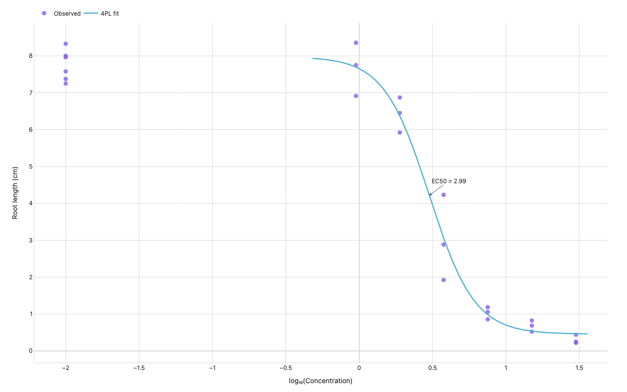
Dose-response curve

Python Code

"""Pharmacology — Dose-response curve (4PL log-logistic)."""


import numpy as np
import pandas as pd
import plotly.graph_objects as go
from scipy.optimize import curve_fit

URL = "https://vincentarelbundock.github.io/Rdatasets/csv/drc/ryegrass.csv"


def four_param_loglogistic(x, bottom, top, ec50, hill):
    """4-parameter log-logistic model. x is actual concentration (not log)."""
    return bottom + (top - bottom) / (1 + (ec50 / np.where(x > 0, x, 1e-9)) ** hill)


def generate():
    print("fetching ryegrass dose-response data …")
    try:
        df = fetch_csv(URL)
        print(f"  cols: {list(df.columns)}")
        # Expected cols: rownames, conc, rootl
        conc_col = next((c for c in df.columns if "conc" in c.lower()), df.columns[-2])
        resp_col = next((c for c in df.columns if "rootl" in c.lower() or "resp" in c.lower()), df.columns[-1])
        df = df[[conc_col, resp_col]].dropna()
        df.columns = ["conc", "rootl"]
        df["conc"] = pd.to_numeric(df["conc"], errors="coerce")
        df["rootl"] = pd.to_numeric(df["rootl"], errors="coerce")
        df = df.dropna()
        used_synthetic = False
    except Exception as e:
        print(f"  fetch failed ({e}); generating synthetic dose-response data")
        used_synthetic = True
        rng = np.random.default_rng(42)
        conc = np.array([0, 0.25, 0.5, 1, 1.5, 2, 3, 4, 5, 10, 15, 20, 30])
        # true params: bottom=0.5, top=7.5, ec50=3.5, hill=2.5
        true_y = four_param_loglogistic(np.where(conc > 0, conc, 1e-9), 0.5, 7.5, 3.5, 2.5)
        noise = rng.normal(0, 0.3, len(conc))
        rootl = np.clip(true_y + noise, 0, None)
        df = pd.DataFrame({"conc": conc, "rootl": rootl})

    # Fit 4PL
    conc_arr = df["conc"].values
    rootl_arr = df["rootl"].values

    # Use nonzero concentrations for fitting
    mask = conc_arr > 0
    x_fit = conc_arr[mask]
    y_fit = rootl_arr[mask]

    try:
        p0 = [rootl_arr.min(), rootl_arr.max(), np.median(x_fit), 2.0]
        popt, _ = curve_fit(
            four_param_loglogistic, x_fit, y_fit,
            p0=p0, maxfev=10000,
            bounds=([0, 0, 0, 0.1], [np.inf, np.inf, np.inf, 20])
        )
        bottom, top, ec50, hill = popt
        print(f"  fit: bottom={bottom:.3f}, top={top:.3f}, EC50={ec50:.3f}, hill={hill:.3f}")

        # Dense grid for fitted curve
        x_dense = np.logspace(np.log10(x_fit.min() * 0.5), np.log10(x_fit.max() * 1.2), 300)
        y_dense = four_param_loglogistic(x_dense, *popt)
        fit_ok = True
    except Exception as fe:
        print(f"  curve_fit failed ({fe}); skipping fit line")
        fit_ok = False

    # Convert to log10 for display
    log_conc = np.log10(conc_arr + 0.01)

    traces = [
        go.Scatter(
            x=log_conc,
            y=rootl_arr,
            mode="markers",
            marker=dict(color=VIOLET, size=9, opacity=0.8),
            name="Observed",
            hovertemplate="log10(conc)=%{x:.2f}<br>root length=%{y:.2f} cm<extra></extra>",
        )
    ]
    annotations = []
    if fit_ok:
        traces.append(go.Scatter(
            x=np.log10(x_dense + 0.01),
            y=y_dense,
            mode="lines",
            line=dict(color=TEAL, width=2.5),
            name="4PL fit",
            hovertemplate="log10(conc)=%{x:.2f}<br>fitted=%{y:.2f} cm<extra></extra>",
        ))
        log_ec50 = np.log10(ec50 + 0.01)
        ec50_y = four_param_loglogistic(ec50, *popt)
        annotations = [
            dict(
                x=log_ec50,
                y=ec50_y,
                text=f"EC50 = {ec50:.2f}",
                showarrow=True,
                arrowhead=2,
                ax=40, ay=-30,
                font=dict(size=12),
            )
        ]

    fig = go.Figure(traces)
    fig.update_layout(
        xaxis=dict(title="log₁₀(Concentration)"),
        yaxis=dict(title="Root length (cm)"),
        legend=dict(orientation="h", y=1.05, x=0),
        annotations=annotations,
        margin=dict(t=40, b=60, l=70, r=40),
        height=500,
    )
    return fig


if __name__ == "__main__":
    generate()

Made with Plotly