Fan chart for CPI YoY inflation with forecast uncertainty bands

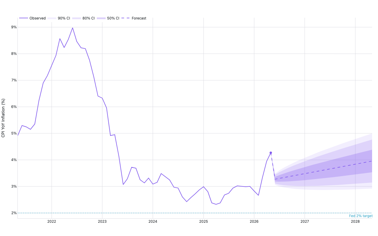
Python Code

"""Macro — Fan chart for CPI YoY inflation with forecast uncertainty bands."""


import numpy as np
import pandas as pd
import plotly.graph_objects as go
import requests
import warnings
warnings.filterwarnings("ignore")


FRED_URL = "https://fred.stlouisfed.org/graph/fredgraph.csv?id=CPIAUCSL"


def fetch_cpi():
    try:
        headers = {"User-Agent": "Mozilla/5.0 (compatible; research)"}
        r = requests.get(FRED_URL, headers=headers, timeout=30, verify=False)
        r.raise_for_status()
        from io import StringIO
        df = pd.read_csv(StringIO(r.text))
        # FRED uses 'observation_date' or 'DATE' depending on API version
        date_col = next((c for c in df.columns if "date" in c.lower()), None)
        val_col = next((c for c in df.columns if "CPI" in c.upper()), None)
        if date_col is None or val_col is None:
            raise ValueError(f"unexpected FRED columns: {df.columns.tolist()}")
        df = df.rename(columns={date_col: "date", val_col: "cpi"})
        df["date"] = pd.to_datetime(df["date"])
        df = df.dropna()
        df = df.sort_values("date").set_index("date")
        if len(df) < 36:
            raise ValueError("insufficient data")
        return df
    except Exception as e:
        print(f"  FRED fetch failed ({e}), using synthetic data")
        return None


def make_synthetic():
    """Synthetic CPI data based on known history."""
    dates = pd.date_range("1947-01-01", "2026-04-01", freq="MS")
    # Approximate CPI level starting ~21 in 1947 to ~315 in 2026
    n = len(dates)
    t = np.linspace(0, 1, n)
    log_cpi = np.log(21) + (np.log(315) - np.log(21)) * t
    # Add some bumps: 1970s inflation, 2021-2022 spike
    bump_70s = np.exp(-((t - 0.35) ** 2) / 0.005) * 0.15
    bump_21 = np.exp(-((t - 0.96) ** 2) / 0.0005) * 0.12
    log_cpi = log_cpi + bump_70s + bump_21
    cpi = np.exp(log_cpi)
    return pd.DataFrame({"cpi": cpi}, index=dates)


def build_fig(df):
    # Compute YoY % change
    yoy = df["cpi"].pct_change(12) * 100
    yoy = yoy.dropna()

    # Use last 5 years of history
    cutoff_hist = yoy.index[-1] - pd.DateOffset(years=5)
    hist = yoy[yoy.index >= cutoff_hist]

    # Last observed date and value
    last_date = hist.index[-1]
    last_val = hist.iloc[-1]

    # Linear trend on the last 2 years for forecast
    recent = yoy[yoy.index >= last_date - pd.DateOffset(years=2)]
    x_num = np.arange(len(recent))
    slope, intercept = np.polyfit(x_num, recent.values, 1)

    # Generate 24 months of forecast
    n_fcast = 24
    fcast_dates = pd.date_range(last_date + pd.DateOffset(months=1), periods=n_fcast, freq="MS")
    x_fcast = np.arange(len(recent), len(recent) + n_fcast)
    central = intercept + slope * x_fcast

    # Uncertainty bands grow with sqrt(time)
    residual_std = float(recent.values.std())
    time_steps = np.arange(1, n_fcast + 1)
    sigma = residual_std * np.sqrt(time_steps / 12)

    # z-scores: 90%, 80%, 50% CI
    z90, z80, z50 = 1.645, 1.282, 0.674

    upper90 = central + z90 * sigma
    lower90 = central - z90 * sigma
    upper80 = central + z80 * sigma
    lower80 = central - z80 * sigma
    upper50 = central + z50 * sigma
    lower50 = central - z50 * sigma

    fig = go.Figure()

    # Historical line
    fig.add_trace(go.Scatter(
        x=hist.index, y=hist.values,
        mode="lines",
        name="Observed",
        line=dict(color=VIOLET, width=2),
        hovertemplate="%{x|%b %Y}: %{y:.1f}%<extra></extra>",
    ))

    # Pin marker at handoff between observed and forecast
    fig.add_trace(go.Scatter(
        x=[last_date], y=[last_val],
        mode="markers",
        marker=dict(color=VIOLET, size=8),
        showlegend=False,
        hoverinfo="skip",
    ))

    # Connect last observed to first forecast point
    connect_x = [last_date] + list(fcast_dates)
    connect_central = [last_val] + list(central)

    # Extend bands to include last observed point (zero width at last_date → smooth connection)
    all_fcast_x = [last_date] + list(fcast_dates)
    upper90e = np.array([last_val] + list(upper90))
    lower90e = np.array([last_val] + list(lower90))
    upper80e = np.array([last_val] + list(upper80))
    lower80e = np.array([last_val] + list(lower80))
    upper50e = np.array([last_val] + list(upper50))
    lower50e = np.array([last_val] + list(lower50))

    # 90% CI band (widest)
    fig.add_trace(go.Scatter(
        x=list(all_fcast_x) + list(all_fcast_x[::-1]),
        y=list(upper90e) + list(lower90e[::-1]),
        fill="toself",
        fillcolor="rgba(132,94,238,0.10)",
        line=dict(color="rgba(0,0,0,0)"),
        name="90% CI",
        hoverinfo="skip",
    ))
    # 80% CI
    fig.add_trace(go.Scatter(
        x=list(all_fcast_x) + list(all_fcast_x[::-1]),
        y=list(upper80e) + list(lower80e[::-1]),
        fill="toself",
        fillcolor="rgba(132,94,238,0.18)",
        line=dict(color="rgba(0,0,0,0)"),
        name="80% CI",
        hoverinfo="skip",
    ))
    # 50% CI
    fig.add_trace(go.Scatter(
        x=list(all_fcast_x) + list(all_fcast_x[::-1]),
        y=list(upper50e) + list(lower50e[::-1]),
        fill="toself",
        fillcolor="rgba(132,94,238,0.28)",
        line=dict(color="rgba(0,0,0,0)"),
        name="50% CI",
        hoverinfo="skip",
    ))

    # Central forecast line
    fig.add_trace(go.Scatter(
        x=connect_x, y=connect_central,
        mode="lines",
        name="Forecast",
        line=dict(color=VIOLET, width=2, dash="dash"),
        hovertemplate="%{x|%b %Y}: %{y:.1f}%<extra></extra>",
    ))

    # 2% Fed target reference
    fig.add_hline(
        y=2.0, line_color=TEAL, line_dash="dot", line_width=1.5,
        annotation_text="Fed 2% target",
        annotation_position="bottom right",
        annotation_font_color=TEAL,
    )

    fig.update_layout(
        
        yaxis_title="CPI YoY Inflation (%)",
        legend=dict(orientation="h", y=1.02, x=0),
        margin=dict(t=60, b=60, l=60, r=20),
        yaxis=dict(ticksuffix="%"),
    )
    return fig


def generate():
    df = fetch_cpi()
    if df is None:
        df = make_synthetic()
        print("  using synthetic CPI data")
    else:
        print(f"  fetched {len(df)} months of CPI data from FRED")
    fig = build_fig(df)
    return fig


if __name__ == "__main__":
    generate()

Made with Plotly