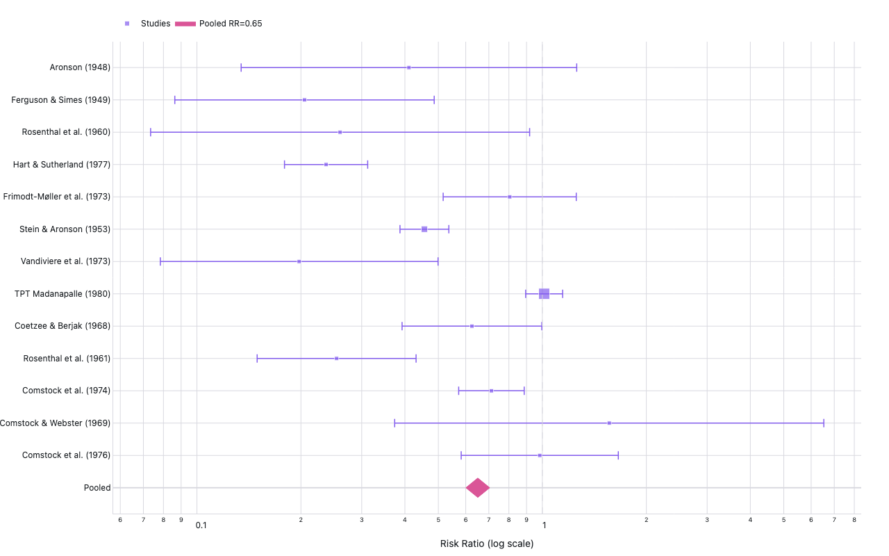
Forest plot

Python Code

"""Forest plot — BCG vaccine vs TB meta-analysis (13 trials)."""


import numpy as np
import pandas as pd
import plotly.graph_objects as go

URL = "https://vincentarelbundock.github.io/Rdatasets/csv/HSAUR/BCG.csv"


def generate():
    print("fetching BCG meta-analysis data …")
    df = fetch_csv(URL)
    df.columns = [c.strip() for c in df.columns]
    print(f"  cols: {list(df.columns)}")

    # Expected cols: BCGTB, BCGVacc, NoVaccTB, NoVacc (plus Trial and possibly other metadata)
    tb_v  = "BCGTB"
    n_v   = "BCGVacc"
    tb_nv = "NoVaccTB"
    n_nv  = "NoVacc"

    # Flexible column matching
    for expected, alts in [(tb_v, ["bcgtb","vacc_tb","treated_tb"]),
                           (n_v, ["bcgvacc","vacc_n","n_treated"]),
                           (tb_nv, ["novacctb","control_tb"]),
                           (n_nv, ["novacc","control_n","n_control"])]:
        if expected not in df.columns:
            match = next((c for c in df.columns if c.lower() in alts), None)
            if match:
                df = df.rename(columns={match: expected})

    print(f"  using cols: {tb_v}, {n_v}, {tb_nv}, {n_nv}")
    df = df.dropna(subset=[tb_v, n_v, tb_nv, n_nv])
    for c in [tb_v, n_v, tb_nv, n_nv]:
        df[c] = pd.to_numeric(df[c], errors="coerce")
    df = df.dropna()

    # Risk ratio per study: RR = (BCGTB/BCGVacc) / (NoVaccTB/NoVacc)
    # log(RR) ± 1.96*SE, SE = sqrt(1/a - 1/n1 + 1/c - 1/n2)
    df["risk_vacc"]   = df[tb_v]  / df[n_v]
    df["risk_novacc"] = df[tb_nv] / df[n_nv]
    df["RR"]          = df["risk_vacc"] / df["risk_novacc"]
    df["logRR"]       = np.log(df["RR"])
    df["SE"]          = np.sqrt(
        1/np.maximum(df[tb_v],1) - 1/np.maximum(df[n_v],1) +
        1/np.maximum(df[tb_nv],1) - 1/np.maximum(df[n_nv],1)
    )
    df["CI_lo"] = np.exp(df["logRR"] - 1.96 * df["SE"])
    df["CI_hi"] = np.exp(df["logRR"] + 1.96 * df["SE"])

    # Pooled (inverse-variance) estimate
    df["weight"] = 1 / df["SE"]**2
    pool_logRR = np.sum(df["weight"] * df["logRR"]) / np.sum(df["weight"])
    pool_SE    = np.sqrt(1 / np.sum(df["weight"]))
    pool_RR    = np.exp(pool_logRR)
    pool_lo    = np.exp(pool_logRR - 1.96 * pool_SE)
    pool_hi    = np.exp(pool_logRR + 1.96 * pool_SE)

    # BCG trial study names (matched by row order in the Rdatasets BCG dataset)
    BCG_STUDY_NAMES = [
        "Aronson (1948)",
        "Ferguson & Simes (1949)",
        "Rosenthal et al. (1960)",
        "Hart & Sutherland (1977)",
        "Frimodt-Møller et al. (1973)",
        "Stein & Aronson (1953)",
        "Vandiviere et al. (1973)",
        "TPT Madanapalle (1980)",
        "Coetzee & Berjak (1968)",
        "Rosenthal et al. (1961)",
        "Comstock et al. (1974)",
        "Comstock & Webster (1969)",
        "Comstock et al. (1976)",
    ]
    if len(df) == len(BCG_STUDY_NAMES):
        labels = BCG_STUDY_NAMES
    else:
        trial_col = next((c for c in df.columns if "trial" in c.lower() or "study" in c.lower() or "author" in c.lower()), None)
        labels = df[trial_col].astype(str).tolist() if trial_col else [f"Trial {i+1}" for i in range(len(df))]

    # Build forest plot (horizontal)
    y_pos = list(range(len(df), 0, -1))   # studies top to bottom

    fig = go.Figure()

    # Study-level points + CI whiskers
    fig.add_trace(go.Scatter(
        x=df["RR"], y=y_pos,
        mode="markers",
        marker=dict(
            color=VIOLET,
            size=[max(6, min(16, w / df["weight"].max() * 16)) for w in df["weight"]],
            symbol="square",
        ),
        error_x=dict(
            type="data",
            symmetric=False,
            array=(df["CI_hi"] - df["RR"]).tolist(),
            arrayminus=(df["RR"] - df["CI_lo"]).tolist(),
            color=VIOLET,
            thickness=1.5,
            width=6,
        ),
        name="Studies",
        hovertemplate="RR=%{x:.2f} [%{customdata[0]:.2f}, %{customdata[1]:.2f}]<extra></extra>",
        customdata=list(zip(df["CI_lo"], df["CI_hi"])),
    ))

    # Pooled diamond
    diamond_x = [pool_lo, pool_RR, pool_hi, pool_RR, pool_lo]
    diamond_y = [0, 0.3, 0, -0.3, 0]
    fig.add_trace(go.Scatter(
        x=diamond_x, y=diamond_y,
        mode="lines", fill="toself",
        fillcolor=PINK, line=dict(color=PINK, width=1),
        name=f"Pooled RR={pool_RR:.2f}",
        hovertemplate=f"Pooled RR={pool_RR:.2f}<extra></extra>",
    ))

    # No-effect line
    fig.add_vline(x=1.0, line=dict(color=GRID, width=1, dash="dash"))

    # Y-axis study labels
    fig.update_layout(
        title=dict(text="Forest Plot — BCG Vaccine vs TB (13 RCTs)", x=0.5),
        xaxis=dict(title="Risk Ratio (log scale)", type="log"),
        yaxis=dict(
            tickvals=y_pos + [0],
            ticktext=labels + ["Pooled"],
            range=[-0.8, len(df) + 0.8],
        ),
        legend=dict(orientation="h", y=1.06),
        margin=dict(t=60, b=60, l=140, r=40),
        height=max(400, len(df) * 28 + 120),
        showlegend=True,
    )
    return fig


if __name__ == "__main__":
    generate()

Made with Plotly