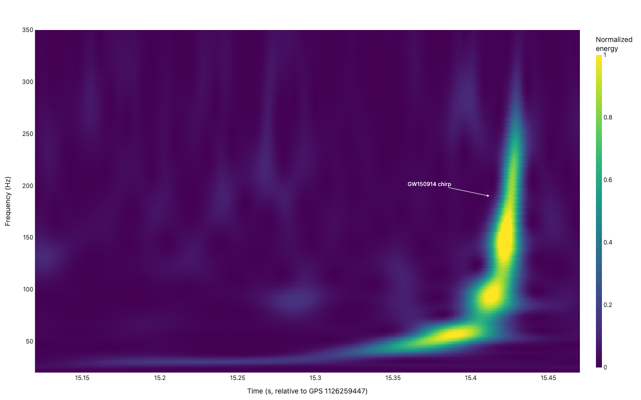
LIGO gravitational-wave spectrogram

Python Code

"""LIGO gravitational-wave spectrogram — H1 strain, GW150914."""


import numpy as np
import plotly.graph_objects as go

LIGO_FILE = Path(__file__).parents[4] / "plotly-studio/qa/super_prompts/data/H-H1_GWOSC_16KHZ_R1-1126259447-32.hdf5"
FS = 16384   # Hz sampling rate of the GWOSC 16 kHz strain file

# GW150914 reached peak strain (merger) at GPS 1126259462.4. The 32-second
# segment in this file starts at GPS 1126259447, so the event sits 15.4 s in.
START_GPS = 1126259447
EVENT_GPS = 1126259462.4
EVENT_T   = EVENT_GPS - START_GPS   # ≈ 15.4 s into the segment


def _load_strain():
    import h5py
    with h5py.File(LIGO_FILE, "r") as f:
        for key in ["strain/Strain", "strain", "data"]:
            try:
                obj = f[key]
                if hasattr(obj, "__len__"):
                    return np.array(obj)
            except KeyError:
                pass
        # Fall back to any long 1-D array
        arrays = []
        f.visititems(lambda name, obj: arrays.append(np.array(obj))
                     if len(getattr(obj, "shape", [])) == 1 and getattr(obj, "shape", [0])[0] > 1000
                     else None)
        if arrays:
            return arrays[0]
    raise RuntimeError("Could not find strain array in LIGO HDF5 file")


def generate():
    print("reading LIGO HDF5 …")
    from scipy import signal
    from scipy.signal import resample_poly

    strain = _load_strain()
    print(f"  strain shape: {strain.shape}, fs={FS} Hz")

    # ── Whiten: flatten the spectrum by dividing by the noise amplitude ───────
    # A plain STFT of the raw strain is dominated by LIGO's coloured detector
    # noise and the chirp is invisible. Whitening (divide by the ASD) plus a
    # band-pass is the standard GW pre-processing that exposes the signal.
    freqs = np.fft.rfftfreq(len(strain), 1 / FS)
    strain_fft = np.fft.rfft(strain)
    f_w, psd = signal.welch(strain, fs=FS, nperseg=4 * FS)
    psd_interp = np.interp(freqs, f_w, psd)
    psd_interp[psd_interp <= 0] = 1e-40
    whitened = np.fft.irfft(strain_fft / np.sqrt(psd_interp), n=len(strain))

    # Band-pass to LIGO's most sensitive band (20–350 Hz), which spans the chirp
    b, a = signal.butter(4, [20, 350], btype="bandpass", fs=FS)
    whitened = signal.filtfilt(b, a, whitened)

    # Down-sample to 2048 Hz — the chirp lives below 350 Hz, and a lower rate
    # makes the wavelet transform far cheaper without losing the signal.
    fs2 = 2048
    wd = resample_poly(whitened, fs2, FS)
    t  = np.arange(len(wd)) / fs2

    # ── Morlet wavelet scalogram (constant-Q) ─────────────────────────────────
    # A fixed-window STFT can't resolve a fast frequency sweep — at the time
    # resolution needed to see the chirp, the frequency bins smear it into the
    # noise. A continuous wavelet transform uses a window that shrinks with
    # frequency, which is exactly how LIGO's own "Q-scan" plots make the chirp
    # pop. Compute on a padded window, then crop so edge artefacts fall offscreen.
    pad = 0.6
    sel = (t >= EVENT_T - pad) & (t <= EVENT_T + 0.35)
    seg, t_seg = wd[sel], t[sel]

    w0 = 8.0
    f_spec = np.linspace(20, 350, 200)
    widths = w0 * fs2 / (2 * np.pi * f_spec)
    power = np.abs(signal.cwt(seg, signal.morlet2, widths, w=w0)) ** 2

    # Crop to a ~0.35 s window around the merger and thin the time axis a little
    d0, d1 = EVENT_T - 0.28, EVENT_T + 0.07
    dm = (t_seg >= d0) & (t_seg <= d1)
    t_spec, Z = t_seg[dm], power[:, dm]
    stride = max(1, Z.shape[1] // 240)
    t_spec, Z = t_spec[::stride], Z[:, ::stride]

    # Normalise to peak energy (the conventional scalogram colour scale) and
    # round to keep the interactive JSON small.
    Z = np.round(Z / np.percentile(Z, 99.7), 3)

    fig = go.Figure(go.Heatmap(
        x=t_spec,
        y=f_spec,
        z=Z,
        colorscale="Viridis",
        zmin=0,
        zmax=1.0,
        colorbar=dict(title="Normalized<br>energy", thickness=12),
        hovertemplate="t=%{x:.3f}s<br>f=%{y:.0f}Hz<br>%{z:.2f}<extra></extra>",
    ))

    # The chirp sweeps up from ~35 Hz to ~250 Hz over the last ~0.2 s before merger
    fig.add_annotation(
        x=EVENT_T + 0.012, y=190,
        ax=-70, ay=-15,
        text="GW150914 chirp",
        showarrow=True, arrowhead=2, arrowcolor="white",
        font=dict(color="white", size=11),
    )

    fig.update_layout(
        title=dict(text="LIGO H1 Spectrogram — GW150914 (whitened + bandpassed)", x=0.5),
        xaxis=dict(title="Time (s, relative to GPS 1126259447)"),
        yaxis=dict(title="Frequency (Hz)", range=[20, 350]),
        margin=dict(t=60, b=50, l=70, r=70),
        height=460,
    )
    return fig


if __name__ == "__main__":
    generate()

Made with Plotly