
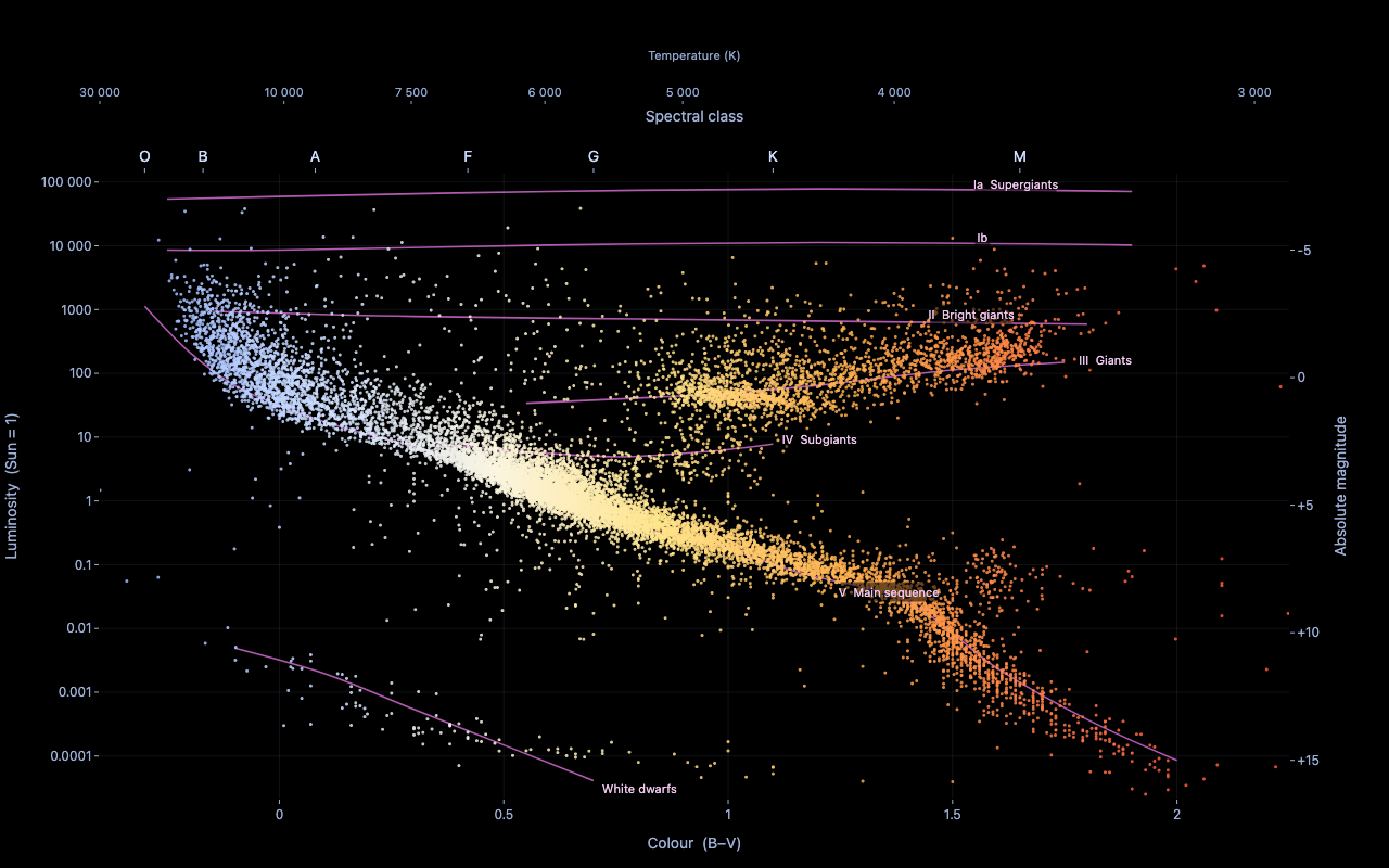
Hertzsprung-Russell diagram
HYG star catalog v4.1
Example from the compendium of canonical charts
Python Code
"""Hertzsprung-Russell diagram — HYG star catalog v4.1.
Styled after the classic dark HR diagram on Wikipedia
(https://en.wikipedia.org/wiki/Hertzsprung-Russell_diagram, File:HRDiagram.png):
black field, four labelled axes (colour + spectral class / temperature on the
horizontal pair, luminosity + absolute magnitude on the vertical pair), and the
luminosity-class bands sketched over the scatter.
"""
from pathlib import Path
# ── Palette + theme (matching the Plotly Studio gallery these charts ship in) ──
VIOLET, TEAL, GREEN, PINK, ORANGE = "#845EEE", "#52B3D0", "#55B685", "#DA5597", "#E9A23B"
PRIMARY, SECONDARY = VIOLET, TEAL
COLORWAY = [VIOLET, TEAL, GREEN, PINK, ORANGE]
BG, TEXT, GRID, MUTED = "#ffffff", "#1c2024", "#d9d9e0", "#60646c"
FONT = "Inter, -apple-system, BlinkMacSystemFont, sans-serif"
COLORSCALE = [[0, "rgba(132, 94, 238, 0.05)"], [1, "rgba(132, 94, 238, 0.9)"]]
def apply_theme(fig):
"""Light gallery theme: white background, Inter font, soft gridlines."""
fig.update_layout(
paper_bgcolor=BG, plot_bgcolor=BG, colorway=COLORWAY,
font=dict(family=FONT, color=TEXT, size=12),
legend=dict(font=dict(color=TEXT)),
hoverlabel=dict(bgcolor="#f0f0f3", font=dict(color=TEXT, family=FONT), bordercolor=GRID),
)
fig.update_xaxes(gridcolor=GRID, linecolor=GRID, zerolinecolor=GRID)
fig.update_yaxes(gridcolor=GRID, linecolor=GRID, zerolinecolor=GRID)
def fetch_csv(url, **kwargs):
import io
import pandas as pd
import requests
r = requests.get(url, timeout=60)
r.raise_for_status()
return pd.read_csv(io.StringIO(r.text), **kwargs)
def fetch_json(url):
import requests
r = requests.get(url, timeout=60)
r.raise_for_status()
return r.json()
import io
import numpy as np
import pandas as pd
import plotly.graph_objects as go
import requests, warnings
URL = "https://raw.githubusercontent.com/astronexus/HYG-Database/master/hyg/CURRENT/hygdata_v41.csv"
# ── Physical conversions ──────────────────────────────────────────────────────
M_SUN = 4.83 # Sun's absolute visual magnitude → luminosity zero-point
def bv_to_temp(bv):
"""Ballesteros (2012) effective temperature from B–V colour index (K)."""
bv = np.asarray(bv, dtype=float)
return 4600.0 * (1.0 / (0.92 * bv + 1.7) + 1.0 / (0.92 * bv + 0.62))
def temp_to_bv(temp):
"""Invert bv_to_temp numerically over the plotted colour range."""
grid = np.linspace(-0.4, 2.4, 4000)
t = bv_to_temp(grid)
order = np.argsort(t)
return float(np.interp(temp, t[order], grid[order]))
def absmag_to_lum(m):
"""Luminosity in solar units from absolute magnitude."""
return 10.0 ** ((M_SUN - np.asarray(m, dtype=float)) / 2.5)
# ── Luminosity-class ridge lines (approximate empirical loci) ─────────────────
# Each is a hand-tabulated polyline in (B–V, absolute magnitude) space.
ZONES = {
"Ia Supergiants": [(-0.25, -7.0), (0.0, -7.1), (0.6, -7.3), (1.2, -7.4), (1.9, -7.3)],
"Ib": [(-0.25, -5.0), (0.0, -5.0), (0.6, -5.2), (1.2, -5.3), (1.9, -5.2)],
"II Bright giants": [(-0.15, -2.6), (0.3, -2.4), (0.8, -2.3), (1.3, -2.2), (1.8, -2.1)],
"III Giants": [(0.55, 1.0), (0.8, 0.8), (1.0, 0.6), (1.2, 0.3), (1.5, -0.3), (1.75, -0.6)],
"IV Subgiants": [(0.35, 2.6), (0.55, 2.9), (0.75, 3.1), (0.95, 2.9), (1.1, 2.6)],
"V Main sequence": [
(-0.30, -2.8), (-0.20, -1.0), (-0.10, 0.3), (0.00, 1.1), (0.15, 2.0),
(0.30, 2.7), (0.45, 3.5), (0.60, 4.5), (0.70, 5.2), (0.81, 5.9),
(1.00, 6.7), (1.15, 7.6), (1.40, 8.8), (1.60, 11.4), (1.80, 13.4), (2.00, 15.0),
],
"White dwarfs": [(-0.10, 10.6), (0.10, 11.6), (0.30, 13.0), (0.50, 14.4), (0.70, 15.8)],
}
# Where to drop each band's text label (B–V, abs mag) and its anchor.
ZONE_LABELS = {
"Ia Supergiants": (1.55, -7.6, "left"),
"Ib": (1.55, -5.5, "left"),
"II Bright giants": (1.45, -2.5, "left"),
"III Giants": (1.78, -0.7, "left"),
"IV Subgiants": (1.12, 2.4, "left"),
"V Main sequence": (1.25, 8.4, "left"),
"White dwarfs": (0.72, 16.1, "left"),
}
LINE_COLOR = "#d36bd0" # magenta ridge lines, as in the reference
AXIS_COLOR = "#9fb0d6" # cool blue-grey for axis lines / ticks on black
LABEL_BG = "rgba(0,0,0,0.55)"
def generate():
print("downloading HYG catalog (full) …")
warnings.filterwarnings("ignore")
requests.packages.urllib3.disable_warnings()
r = requests.get(URL, verify=False, timeout=180)
r.raise_for_status()
df = pd.read_csv(io.BytesIO(r.content), low_memory=False)
print(f" raw rows: {len(df)}")
for c in ("ci", "absmag", "mag", "dist"):
df[c] = pd.to_numeric(df[c], errors="coerce")
df = df.dropna(subset=["ci", "absmag"])
# Combine a bright (apparent mag) sample — which fills the upper main
# sequence, giants and supergiants — with a nearby volume-limited sample,
# which supplies the faint lower main sequence and white dwarfs the bright
# cut alone would miss. Together they trace the full HR sweep.
bright = df[df["mag"] < 6.5]
nearby = df[df["dist"] < 75]
stars = pd.concat([bright, nearby]).drop_duplicates(subset="id")
if len(stars) > 14000:
stars = stars.sample(14000, random_state=7)
print(f" plotted stars: {len(stars)} (bright {len(bright)}, nearby {len(nearby)})")
temp = bv_to_temp(stars["ci"])
lum = absmag_to_lum(stars["absmag"])
names = stars["proper"].fillna("").astype(str)
names = names.mask(names.eq(""), "—")
customdata = np.column_stack([
names,
stars["spect"].fillna("—").astype(str),
temp,
lum,
stars["absmag"],
stars["ci"],
stars["dist"].fillna(np.nan),
stars["con"].fillna("—").astype(str),
])
hover = (
"<b>%{customdata[0]}</b>"
"<br>Spectral type %{customdata[1]}"
"<br>Temperature %{customdata[2]:,.0f} K"
"<br>Luminosity %{customdata[3]:.3g} L<sub>☉</sub>"
"<br>Abs. magnitude %{customdata[4]:.2f}"
"<br>Colour (B–V) %{customdata[5]:.2f}"
"<br>Distance %{customdata[6]:.1f} pc"
"<br>Constellation %{customdata[7]}"
"<extra></extra>"
)
fig = go.Figure()
# ── Luminosity-class ridge lines ──────────────────────────────────────────
for name, pts in ZONES.items():
xs, ys = zip(*pts)
fig.add_trace(go.Scatter(
x=xs, y=ys, mode="lines",
line=dict(color=LINE_COLOR, width=1.6, shape="spline"),
opacity=0.85, hoverinfo="skip", showlegend=False,
))
# ── Stars ────────────────────────────────────────────────────────────────
fig.add_trace(go.Scattergl(
x=stars["ci"], y=stars["absmag"], mode="markers",
marker=dict(
color=stars["ci"],
colorscale=[
[0.00, "#9bb8ff"], # blue-white (hot O/B)
[0.18, "#cfe0ff"], # white (A)
[0.34, "#fbf5e0"], # yellow-white (F)
[0.50, "#ffe48a"], # yellow (G)
[0.68, "#ffb04d"], # orange (K)
[1.00, "#ff5a3c"], # red (M)
],
cmin=-0.3, cmax=2.0,
size=3, opacity=0.85,
line=dict(width=0),
showscale=False,
),
customdata=customdata,
hovertemplate=hover,
showlegend=False,
))
# Invisible anchor traces: an overlaying axis only renders its ticks when a
# trace is assigned to it, so give the two top axes one transparent point each.
for ax in ("x2", "x3"):
fig.add_trace(go.Scatter(
x=[-0.3, 1.6], y=[0, 0], xaxis=ax, yaxis="y",
mode="markers", marker=dict(opacity=0),
hoverinfo="skip", showlegend=False,
))
fig.add_trace(go.Scatter(
x=[0, 0], y=[0, 10], xaxis="x", yaxis="y2",
mode="markers", marker=dict(opacity=0),
hoverinfo="skip", showlegend=False,
))
# ── Axis tick maps ─────────────────────────────────────────────────────────
# Vertical: plot absolute magnitude (left axis relabelled as luminosity,
# right axis kept as magnitude). A linear magnitude scale *is* a log
# luminosity scale, so the powers-of-ten luminosity ticks land on a grid.
lum_powers = [1e5, 1e4, 1e3, 1e2, 10, 1, 0.1, 1e-2, 1e-3, 1e-4]
lum_labels = ["100 000", "10 000", "1000", "100", "10", "1",
"0.1", "0.01", "0.001", "0.0001"]
lum_tickvals = [M_SUN - 2.5 * np.log10(p) for p in lum_powers]
y_range = [16.5, -8.0] # faint (bottom) → bright (top)
mag_ticks = [-5, 0, 5, 10, 15]
# Horizontal: colour on the bottom; spectral class and temperature stacked
# on top, all sharing the colour range.
x_range = [-0.4, 2.25]
spectral = [("O", -0.30), ("B", -0.17), ("A", 0.08), ("F", 0.42),
("G", 0.70), ("K", 1.10), ("M", 1.65)]
spec_vals = [bv for _, bv in spectral]
spec_text = [s for s, _ in spectral]
temps = [30000, 10000, 7500, 6000, 5000, 4000, 3000]
temp_vals = [temp_to_bv(t) for t in temps]
temp_text = [f"{t:,}".replace(",", " ") for t in temps]
# Reserve vertical room above the plot for the two stacked top axes.
PLOT_TOP = 0.90
fig.update_layout(
paper_bgcolor="#000000",
plot_bgcolor="#000000",
font=dict(family=FONT, color=AXIS_COLOR, size=12),
margin=dict(t=96, b=64, l=92, r=92),
autosize=True, # interactive chart fills its container; PNG size set in to_image()
showlegend=False,
hoverlabel=dict(
bgcolor="rgba(10,12,24,0.92)",
bordercolor=AXIS_COLOR,
font=dict(color="#e8edf7", family=FONT, size=12),
align="left",
),
# Bottom: colour (B–V)
xaxis=dict(
title=dict(text="Colour (B–V)", font=dict(color=AXIS_COLOR)),
range=x_range, domain=[0, 1], anchor="y",
color=AXIS_COLOR, zeroline=False,
gridcolor="rgba(159,176,214,0.10)", showgrid=True,
ticks="outside", tickcolor=AXIS_COLOR, ticklen=4,
),
# Top inner: spectral class
xaxis2=dict(
title=dict(text="Spectral class", font=dict(color=AXIS_COLOR)),
range=x_range, overlaying="x", side="top", anchor="y",
tickvals=spec_vals, ticktext=spec_text,
tickfont=dict(size=14, color="#cfe0ff"),
showgrid=False, zeroline=False,
ticks="outside", tickcolor=AXIS_COLOR, ticklen=4,
),
# Top outer: temperature
xaxis3=dict(
title=dict(text="Temperature (K)", font=dict(color="#8fa6cf", size=11)),
range=x_range, overlaying="x", side="top",
anchor="free", position=1.0,
tickvals=temp_vals, ticktext=temp_text,
tickfont=dict(size=11, color="#8fa6cf"),
showgrid=False, zeroline=False,
ticks="outside", tickcolor="#8fa6cf", ticklen=3,
),
# Left: luminosity (Sun = 1)
yaxis=dict(
title=dict(text="Luminosity (Sun = 1)", font=dict(color=AXIS_COLOR)),
range=y_range, domain=[0, PLOT_TOP], anchor="x",
tickvals=lum_tickvals, ticktext=lum_labels,
color=AXIS_COLOR, zeroline=False,
gridcolor="rgba(159,176,214,0.10)", showgrid=True,
ticks="outside", tickcolor=AXIS_COLOR, ticklen=4,
),
# Right: absolute magnitude
yaxis2=dict(
title=dict(text="Absolute magnitude", font=dict(color=AXIS_COLOR)),
range=y_range, overlaying="y", side="right", anchor="x",
tickvals=mag_ticks, ticktext=[f"{m:+d}".replace("+0", "0") for m in mag_ticks],
color=AXIS_COLOR, zeroline=False, showgrid=False,
ticks="outside", tickcolor=AXIS_COLOR, ticklen=4,
),
)
# ── Zone labels (with their own background, per the reference) ────────────
annotations = []
for name, (x, y, anchor) in ZONE_LABELS.items():
annotations.append(dict(
x=x, y=y, xref="x", yref="y", text=name, showarrow=False,
xanchor=anchor, font=dict(size=11, color="#f0c8ee"),
bgcolor=LABEL_BG, borderpad=2,
))
fig.update_layout(annotations=annotations)
# ── Write outputs (custom save: the site's light theme doesn't apply on a
# deliberately black chart) ────────────────────────────────────────────────
return fig
fig = generate()
fig.show()Made with Plotly