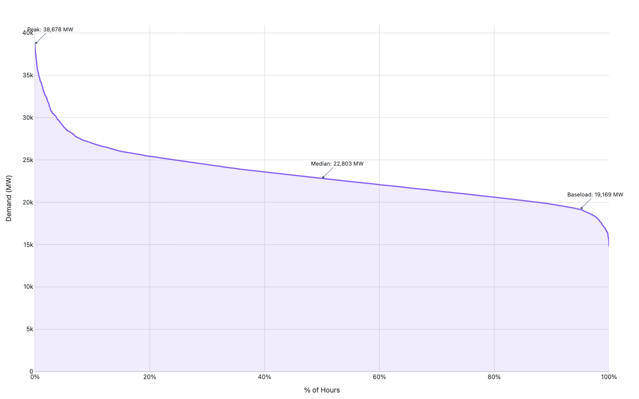
load-duration curve for California (CAISO) grid

Python Code

"""Power Systems — load-duration curve for California (CAISO) grid."""
import io


import numpy as np
import pandas as pd
import plotly.graph_objects as go


# EIA 930 balance file — filter for CISO respondent
EIA_URL = "https://www.eia.gov/electricity/gridmonitor/sixMonthFiles/EIA930_BALANCE_2024_Jan_Jun.csv"


def build_ldc(demand_mw):
    """Return (pct_hours, demand_sorted_desc)."""
    ds = np.sort(demand_mw)[::-1]
    pct = np.linspace(0, 100, len(ds))
    return pct, ds


def generate():
    try:
        print("fetching EIA 930 balance CSV (large file, may take a moment) …")
        import requests
        r = requests.get(EIA_URL, verify=False, timeout=120, stream=True)
        r.raise_for_status()

        # Stream and collect in memory
        content = r.content
        print(f"  downloaded {len(content)//1024//1024} MB")

        df = pd.read_csv(io.BytesIO(content), low_memory=False)
        df.columns = [c.strip() for c in df.columns]
        print(f"  full file: {len(df)} rows; columns sample: {list(df.columns[:8])}")

        # Find respondent / balancing authority column
        resp_col = next(
            (c for c in df.columns if any(k in c.lower() for k in ("respondent", "balancing authority", "ba_code", "balancing_authority"))),
            None
        )
        if resp_col is None:
            raise ValueError(f"No respondent column found. Columns: {list(df.columns)}")

        # Filter CISO (California ISO) — EIA 930 uses "California ISO"
        ciso_mask = (
            df[resp_col].astype(str).str.strip().str.upper().isin(["CISO", "CAISO"]) |
            df[resp_col].astype(str).str.strip().str.lower().str.contains("california")
        )
        ciso = df[ciso_mask]
        print(f"  CISO rows: {len(ciso)}")
        if len(ciso) < 100:
            raise ValueError("Too few CISO rows")

        # Find demand column
        demand_col = next(
            (c for c in ciso.columns if "demand" in c.lower() and "forecast" not in c.lower()),
            None
        )
        if demand_col is None:
            raise ValueError(f"No demand column found. Columns: {list(ciso.columns)}")

        demand = pd.to_numeric(ciso[demand_col], errors="coerce").dropna()
        demand = demand[demand > 0].values
        label = "CAISO (CA) — Jan–Jun 2024"
        source = "EIA-930 Balance"

    except Exception as e:
        print(f"  EIA fetch failed ({e}); using synthetic California-like LDC")
        np.random.seed(13)
        n = 4380  # 6 months of hourly data
        # Bimodal: summer peak demand ~50 GW, winter ~35 GW, base ~25 GW
        base = 28000
        t = np.linspace(0, 2 * np.pi, n)
        seasonal = 8000 * np.sin(t)
        diurnal  = 5000 * np.abs(np.sin(t * 365 / 2))
        noise    = np.random.normal(0, 1200, n)
        demand   = base + seasonal + diurnal + noise
        demand   = np.maximum(demand, 15000)
        label    = "California (synthetic)"
        source   = "Synthetic"

    pct, ds = build_ldc(demand)

    # Annotate key points
    p_peak = ds[0]
    p_base = ds[-1]
    p_med  = ds[len(ds)//2]

    fig = go.Figure()

    fig.add_trace(go.Scatter(
        x=pct, y=ds,
        mode="lines",
        line=dict(color=VIOLET, width=2.5),
        fill="tozeroy",
        fillcolor="rgba(132,94,238,0.12)",
        name=label,
        hovertemplate="%{x:.1f}% of hours<br>%{y:,.0f} MW<extra></extra>",
    ))

    # Annotations
    for pct_ann, val, text in [
        (0,   p_peak, f"Peak: {p_peak:,.0f} MW"),
        (50,  p_med,  f"Median: {p_med:,.0f} MW"),
        (95,  ds[int(0.95*len(ds))], f"Baseload: {ds[int(0.95*len(ds))]:,.0f} MW"),
    ]:
        fig.add_annotation(
            x=pct_ann, y=val, text=text,
            showarrow=True, arrowhead=2,
            ax=30, ay=-30,
            font=dict(size=11),
        )

    fig.update_layout(
        xaxis=dict(title="% of Hours", ticksuffix="%", range=[0, 100]),
        yaxis=dict(title="Demand (MW)"),
        legend=dict(x=0.98, y=0.98, xanchor="right", yanchor="top"),
        margin=dict(t=50, b=50, l=70, r=60),
    )
    return fig


if __name__ == "__main__":
    generate()

Made with Plotly