Lorenz attractor

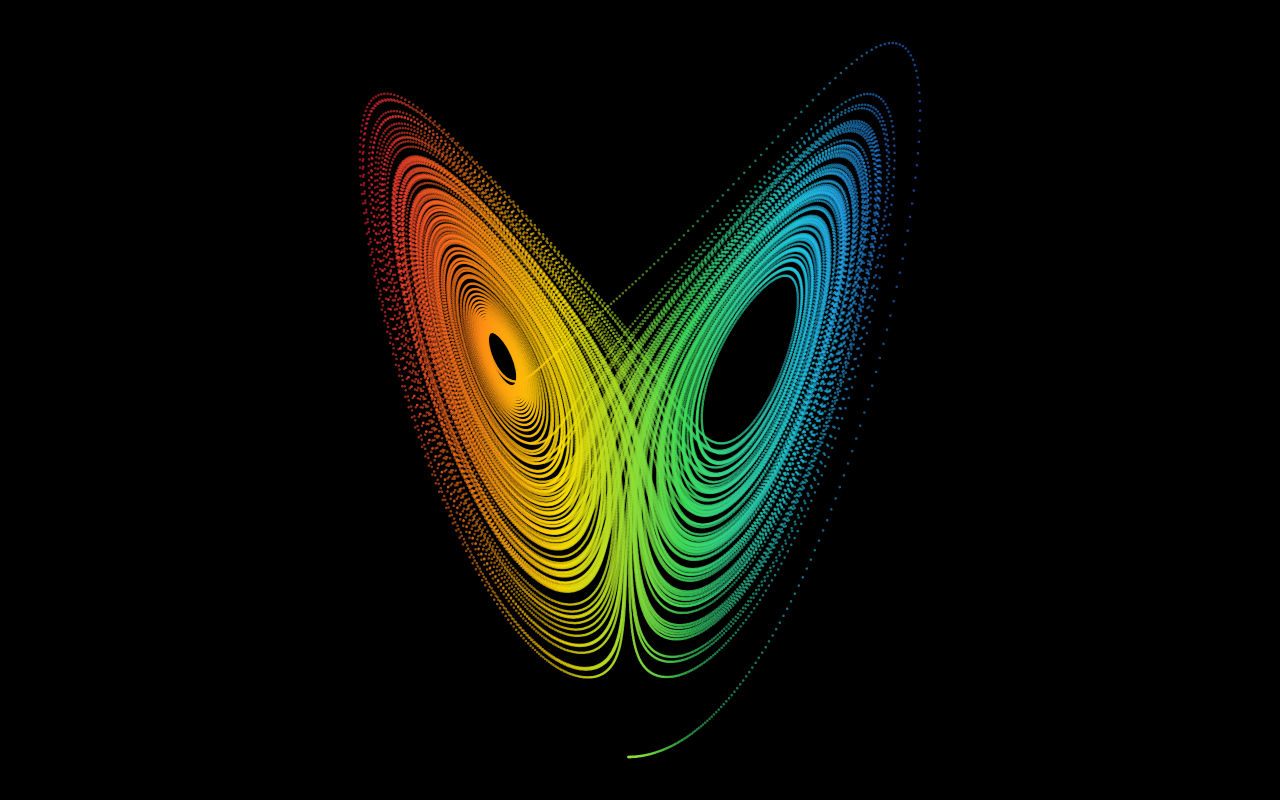
Python Code

"""Dynamical Systems — Lorenz attractor (σ=10, ρ=28, β=8/3)."""
from pathlib import Path

# ── Palette + theme (matching the Plotly Studio gallery these charts ship in) ──
VIOLET, TEAL, GREEN, PINK, ORANGE = "#845EEE", "#52B3D0", "#55B685", "#DA5597", "#E9A23B"
PRIMARY, SECONDARY = VIOLET, TEAL
COLORWAY = [VIOLET, TEAL, GREEN, PINK, ORANGE]
BG, TEXT, GRID, MUTED = "#ffffff", "#1c2024", "#d9d9e0", "#60646c"
FONT = "Inter, -apple-system, BlinkMacSystemFont, sans-serif"
COLORSCALE = [[0, "rgba(132, 94, 238, 0.05)"], [1, "rgba(132, 94, 238, 0.9)"]]


def apply_theme(fig):
    """Light gallery theme: white background, Inter font, soft gridlines."""
    fig.update_layout(
        paper_bgcolor=BG, plot_bgcolor=BG, colorway=COLORWAY,
        font=dict(family=FONT, color=TEXT, size=12),
        legend=dict(font=dict(color=TEXT)),
        hoverlabel=dict(bgcolor="#f0f0f3", font=dict(color=TEXT, family=FONT), bordercolor=GRID),
    )
    fig.update_xaxes(gridcolor=GRID, linecolor=GRID, zerolinecolor=GRID)
    fig.update_yaxes(gridcolor=GRID, linecolor=GRID, zerolinecolor=GRID)


def fetch_csv(url, **kwargs):
    import io
    import pandas as pd
    import requests
    r = requests.get(url, timeout=60)
    r.raise_for_status()
    return pd.read_csv(io.StringIO(r.text), **kwargs)


def fetch_json(url):
    import requests
    r = requests.get(url, timeout=60)
    r.raise_for_status()
    return r.json()

import numpy as np
import plotly.graph_objects as go
from scipy.integrate import solve_ivp


SIGMA, RHO, BETA = 10.0, 28.0, 8.0 / 3.0

# Full-spectrum rainbow, swept left → right across the attractor.
RAINBOW = [
    [0.00, "#ff1f3d"],   # red
    [0.18, "#ff7a18"],   # orange
    [0.36, "#ffe000"],   # yellow
    [0.58, "#3ddc5b"],   # green
    [0.78, "#1fc8e0"],   # cyan
    [1.00, "#2b6bff"],   # blue
]


def lorenz(t, state):
    x, y, z = state
    return [
        SIGMA * (y - x),
        x * (RHO - z) - y,
        x * y - BETA * z,
    ]


def generate():
    print("integrating Lorenz attractor …")

    # One long orbit — the strange attractor is dense enough that a single
    # trajectory, drawn as a haze of translucent points, fills out the set.
    ic = [0.1, 0.0, 0.0]
    t_span = (0, 130)
    t_eval = np.linspace(0, 130, 55000)

    sol = solve_ivp(lorenz, t_span, ic, t_eval=t_eval, rtol=1e-9, atol=1e-11)
    x, y, z = np.round(sol.y, 2)

    print(f"  integrated {len(x)} points, x range [{x.min():.1f}, {x.max():.1f}]")

    fig = go.Figure()

    # Classic (x, z) butterfly silhouette as a glowing point cloud: tiny
    # semi-transparent markers accumulate into smooth luminous ribbons, and the
    # spectrum sweeps across x so the wings run red → blue.
    fig.add_trace(go.Scattergl(
        x=x, y=z,
        mode="markers",
        marker=dict(
            size=2.8,
            color=x,
            colorscale=RAINBOW,
            opacity=0.55,
            showscale=False,
            line=dict(width=0),
        ),
        hoverinfo="skip",
        name="Lorenz attractor",
    ))

    axis = dict(visible=False, showgrid=False, zeroline=False,
                showticklabels=False)
    fig.update_layout(
        xaxis=axis,
        yaxis=dict(visible=False, showgrid=False, zeroline=False,
                   showticklabels=False, scaleanchor="x", scaleratio=1),
        paper_bgcolor="#000000",
        plot_bgcolor="#000000",
        showlegend=False,
        margin=dict(t=0, b=0, l=0, r=0),
        height=800,
    )

    apply_theme(fig)
    return fig


fig = generate()
fig.show()

Made with Plotly