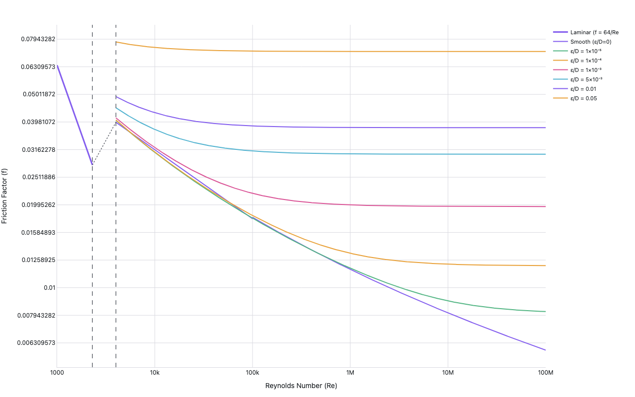
Moody Diagram

Python Code

"""Fluid Mechanics — Moody Diagram (friction factor vs. Reynolds number)."""


import numpy as np
import plotly.graph_objects as go


# Roughness ratios ε/D with display labels
ROUGHNESS = [
    (0,      "Smooth (ε/D=0)"),
    (1e-5,   "ε/D = 1×10⁻⁵"),
    (1e-4,   "ε/D = 1×10⁻⁴"),
    (1e-3,   "ε/D = 1×10⁻³"),
    (5e-3,   "ε/D = 5×10⁻³"),
    (0.01,   "ε/D = 0.01"),
    (0.05,   "ε/D = 0.05"),
]

COLORS = [VIOLET, GREEN, ORANGE, PINK, TEAL, "#845EEE", "#E9A23B"]


def haaland(eps_D, Re):
    """Haaland explicit approximation of Colebrook-White friction factor."""
    return (-1.8 * np.log10((eps_D / 3.7) ** 1.11 + 6.9 / Re)) ** (-2)


def smooth_turbulent(Re):
    """Blasius (Re<1e5) and Prandtl smooth pipe for higher Re."""
    f = np.where(Re < 1e5, 0.316 * Re ** (-0.25), 0.0)
    # Prandtl smooth: 1/sqrt(f) = 2*log10(Re*sqrt(f)) - 0.8 → iterate
    mask = Re >= 1e5
    if mask.any():
        Re_h = Re[mask]
        f_h = 0.316 * Re_h ** (-0.25)  # initial guess
        for _ in range(30):
            f_h = (2.0 * np.log10(Re_h * np.sqrt(f_h)) - 0.8) ** (-2)
        f[mask] = f_h
    return f


def generate():
    Re_turb = np.logspace(np.log10(4000), 8, 600)
    Re_lam = np.logspace(3, np.log10(2300), 100)
    f_lam = 64.0 / Re_lam

    # Transition zone connector (dashed / faint)
    Re_trans = np.array([2300, 4000])
    f_trans_start = 64.0 / 2300
    # Turbulent at Re=4000 for smooth pipe
    f_trans_end = smooth_turbulent(np.array([4000.0]))[0]

    fig = go.Figure()

    # Laminar line
    fig.add_trace(go.Scatter(
        x=Re_lam,
        y=f_lam,
        mode="lines",
        line=dict(color=VIOLET, width=3),
        name="Laminar (f = 64/Re)",
        hovertemplate="Re=%{x:.0f}<br>f=%{y:.5f}<extra></extra>",
    ))

    # Transition zone (dotted)
    fig.add_trace(go.Scatter(
        x=Re_trans,
        y=[f_trans_start, f_trans_end],
        mode="lines",
        line=dict(color=MUTED, width=1.5, dash="dot"),
        name="Transition zone",
        hoverinfo="skip",
        showlegend=False,
    ))

    # Turbulent curves per roughness
    for i, (eps_D, label) in enumerate(ROUGHNESS):
        color = COLORS[i % len(COLORS)]
        if eps_D == 0:
            f_turb = smooth_turbulent(Re_turb)
        else:
            f_turb = haaland(eps_D, Re_turb)
        # Fully rough asymptote: at very high Re, f = (1/(2*log10(3.7/eps_D)))^2
        if eps_D > 0:
            f_fully_rough = (1 / (-2 * np.log10(eps_D / 3.7))) ** 2
            # Clip to fully rough value
            f_turb = np.maximum(f_turb, f_fully_rough * 0.98)

        fig.add_trace(go.Scatter(
            x=Re_turb,
            y=f_turb,
            mode="lines",
            line=dict(color=color, width=2),
            name=label,
            hovertemplate=f"{label}<br>Re=%{{x:.2e}}<br>f=%{{y:.5f}}<extra></extra>",
        ))

    # Vertical lines for transition boundaries
    for Re_v, label_v, dash in [(2300, "Re = 2300<br>(laminar→transition)", "dash"),
                                  (4000, "Re = 4000<br>(transition→turbulent)", "dash")]:
        fig.add_vline(
            x=Re_v,
            line=dict(color=MUTED, width=1.5, dash=dash),
            annotation_text=label_v,
            annotation_position="top right" if Re_v == 2300 else "top left",
            annotation_font=dict(size=10, color=MUTED),
        )

    fig.update_layout(
        xaxis=dict(
            title="Reynolds Number (Re)",
            type="log",
            dtick=1,
            gridcolor="#d9d9e0",
        ),
        yaxis=dict(
            title="Friction Factor (f)",
            type="log",
            dtick=0.1,
            gridcolor="#d9d9e0",
        ),
        legend=dict(x=1.01, y=1.0, xanchor="left", yanchor="top", font=dict(size=11)),
        margin=dict(t=50, b=60, l=70, r=180),
    )

    return fig


if __name__ == "__main__":
    generate()

Made with Plotly