MOSFET I-V curves

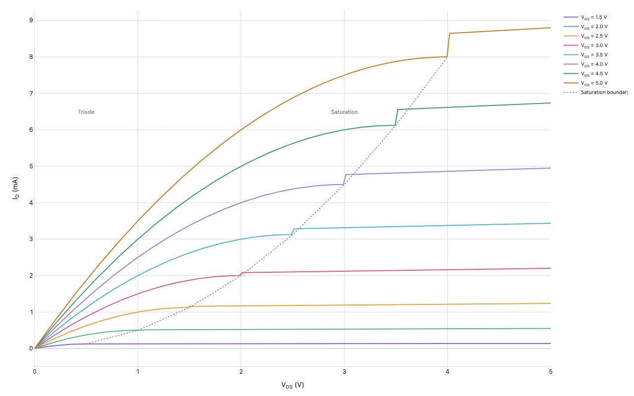
Python Code

"""Device Characterization — MOSFET I-V curves (SPICE Level-1 model, computed)."""
from pathlib import Path

# ── Palette + theme (matching the Plotly Studio gallery these charts ship in) ──
VIOLET, TEAL, GREEN, PINK, ORANGE = "#845EEE", "#52B3D0", "#55B685", "#DA5597", "#E9A23B"
PRIMARY, SECONDARY = VIOLET, TEAL
COLORWAY = [VIOLET, TEAL, GREEN, PINK, ORANGE]
BG, TEXT, GRID, MUTED = "#ffffff", "#1c2024", "#d9d9e0", "#60646c"
FONT = "Inter, -apple-system, BlinkMacSystemFont, sans-serif"
COLORSCALE = [[0, "rgba(132, 94, 238, 0.05)"], [1, "rgba(132, 94, 238, 0.9)"]]


def apply_theme(fig):
    """Light gallery theme: white background, Inter font, soft gridlines."""
    fig.update_layout(
        paper_bgcolor=BG, plot_bgcolor=BG, colorway=COLORWAY,
        font=dict(family=FONT, color=TEXT, size=12),
        legend=dict(font=dict(color=TEXT)),
        hoverlabel=dict(bgcolor="#f0f0f3", font=dict(color=TEXT, family=FONT), bordercolor=GRID),
    )
    fig.update_xaxes(gridcolor=GRID, linecolor=GRID, zerolinecolor=GRID)
    fig.update_yaxes(gridcolor=GRID, linecolor=GRID, zerolinecolor=GRID)


def fetch_csv(url, **kwargs):
    import io
    import pandas as pd
    import requests
    r = requests.get(url, timeout=60)
    r.raise_for_status()
    return pd.read_csv(io.StringIO(r.text), **kwargs)


def fetch_json(url):
    import requests
    r = requests.get(url, timeout=60)
    r.raise_for_status()
    return r.json()

import numpy as np
import plotly.graph_objects as go


def generate():
    # SPICE Level-1 MOSFET parameters
    k   = 1e-3   # process gain (A/V²)
    Vth = 1.0    # threshold voltage (V)
    lam = 0.02   # channel-length modulation (V⁻¹)

    VGS_vals = [1.5, 2.0, 2.5, 3.0, 3.5, 4.0, 4.5, 5.0]
    VDS = np.linspace(0, 5, 200)

    colors = [
        "#845EEE", "#55B685", "#E9A23B", "#DA5597", "#52B3D0",
        "#a07fd6", "#3d9c6e", "#c87c22",
    ]

    fig = go.Figure()

    for idx, vgs in enumerate(VGS_vals):
        ID = np.zeros_like(VDS)
        vov = vgs - Vth  # overdrive voltage

        if vov <= 0:
            # Cutoff: ID = 0 everywhere
            pass
        else:
            for j, vds in enumerate(VDS):
                if vds < vov:
                    # Triode (linear) region
                    ID[j] = k * (vov * vds - vds**2 / 2)
                else:
                    # Saturation region
                    ID[j] = (k / 2) * vov**2 * (1 + lam * vds)

        # Convert A → mA
        ID_mA = ID * 1e3

        fig.add_trace(go.Scatter(
            x=VDS,
            y=ID_mA,
            mode="lines",
            name=f"V<sub>GS</sub> = {vgs:.1f} V",
            line=dict(color=colors[idx % len(colors)], width=2),
            hovertemplate=f"VGS={vgs:.1f}V<br>VDS=%{{x:.2f}}V<br>ID=%{{y:.2f}}mA<extra></extra>",
        ))

    # Boundary between triode and saturation: VDS = VGS - Vth
    vgs_arr = np.array(VGS_vals)
    vds_sat = vgs_arr - Vth
    id_sat_mA = (k / 2) * (vgs_arr - Vth)**2 * 1e3

    # Only show for VGS > Vth
    mask = vgs_arr > Vth
    fig.add_trace(go.Scatter(
        x=vds_sat[mask],
        y=id_sat_mA[mask],
        mode="lines",
        line=dict(color="gray", width=1.5, dash="dot"),
        name="Saturation boundary",
        hovertemplate="VDS<sub>sat</sub>=%{x:.2f}V<br>ID=%{y:.2f}mA<extra></extra>",
    ))

    # Annotations for regions
    fig.add_annotation(
        x=0.5, y=6.5,
        text="Triode",
        showarrow=False,
        font=dict(size=11, color="gray"),
    )
    fig.add_annotation(
        x=3.0, y=6.5,
        text="Saturation",
        showarrow=False,
        font=dict(size=11, color="gray"),
    )

    fig.update_layout(
        xaxis=dict(title="V<sub>DS</sub> (V)", range=[0, 5]),
        yaxis=dict(title="I<sub>D</sub> (mA)", range=[0, None]),
        legend=dict(
            x=1.02, y=1.0,
            xanchor="left",
            font=dict(size=10),
        ),
        margin=dict(t=20, b=60, l=70, r=140),
    )

    apply_theme(fig)
    return fig


fig = generate()
fig.show()

Made with Plotly