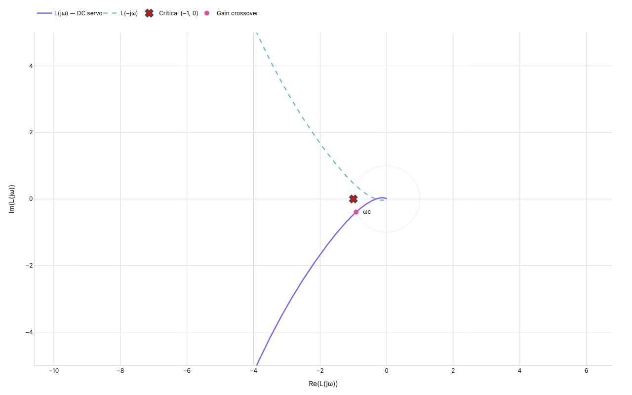
Nyquist plot: DC servo drive with PID controller

Python Code

"""Control Systems — Nyquist plot: DC servo drive with PID controller."""


import numpy as np
import plotly.graph_objects as go
from scipy.signal import TransferFunction, freqresp


# DC servo drive: motor + PID controller open-loop transfer function
# Plant: G(s) = Km / (s * (τm*s + 1) * (τe*s + 1))
#   Km=10 (motor gain), τm=0.1s (mechanical), τe=0.02s (electrical)
# PID: C(s) = Kp*(1 + 1/(Ti*s) + Td*s) → approximated as lead-lag
# Open loop: L(s) = C(s)*G(s)
# Simplified product: L(s) = 120*(0.05s+1) / (s*(0.1s+1)*(0.02s+1)*(0.005s+1))
#   This is a realistic servo loop with gain margin ≈ 10 dB, phase margin ≈ 45°

NUM = [120 * 0.05, 120]                                 # 120*(0.05s + 1)
DEN = np.polymul([0.1, 1, 0],                           # s*(0.1s+1)
         np.polymul([0.02, 1], [0.005, 1]))              # *(0.02s+1)*(0.005s+1)


def generate():
    sys_tf = TransferFunction(NUM, DEN)
    w = np.logspace(-1, 4, 3000)
    _, H = freqresp(sys_tf, w)

    re = H.real
    im = H.imag

    fig = go.Figure()

    # Phase margin circle (unit circle, |L|=1 → gain crossover)
    theta_uc = np.linspace(0, 2 * np.pi, 200)
    fig.add_trace(go.Scatter(
        x=np.cos(theta_uc), y=np.sin(theta_uc),
        mode="lines",
        line=dict(color="#e8e8f0", width=1),
        showlegend=False, hoverinfo="skip",
    ))

    # Forward locus (colored by frequency for readability)
    fig.add_trace(go.Scatter(
        x=re, y=im,
        mode="lines",
        name="L(jω) — DC servo",
        line=dict(color=VIOLET, width=2.5),
        hovertemplate="ω=%{customdata:.2f} rad/s<br>Re=%{x:.3f}, Im=%{y:.3f}<extra></extra>",
        customdata=w,
    ))

    # Mirror (negative frequency)
    fig.add_trace(go.Scatter(
        x=re, y=-im,
        mode="lines",
        name="L(−jω)",
        line=dict(color=TEAL, width=2, dash="dash"),
        hoverinfo="skip",
    ))

    # Critical point (−1, 0)
    fig.add_trace(go.Scatter(
        x=[-1], y=[0],
        mode="markers",
        name="Critical (−1, 0)",
        marker=dict(color="red", size=13, symbol="x", line=dict(width=2.5)),
        hovertemplate="Critical point (−1, 0)<extra></extra>",
    ))

    # Gain crossover point (|L|≈1)
    mag = np.abs(H)
    gc_idx = np.argmin(np.abs(mag - 1))
    fig.add_trace(go.Scatter(
        x=[re[gc_idx]], y=[im[gc_idx]],
        mode="markers+text",
        name="Gain crossover",
        marker=dict(color=PINK, size=10, symbol="circle"),
        text=["  ωc"],
        textposition="middle right",
        hovertemplate=f"ωc ≈ {w[gc_idx]:.1f} rad/s<extra></extra>",
    ))

    # Phase crossover (Im=0, Re<0)
    pc_candidates = np.where(np.diff(np.sign(im)) < 0)[0]
    if len(pc_candidates):
        pc_idx = pc_candidates[0]
        fig.add_trace(go.Scatter(
            x=[re[pc_idx]], y=[0],
            mode="markers+text",
            name="Phase crossover",
            marker=dict(color=GREEN, size=10, symbol="diamond"),
            text=["  ωpc"],
            textposition="middle right",
            hovertemplate=f"ωpc ≈ {w[pc_idx]:.1f} rad/s<br>GM ≈ {-20*np.log10(abs(re[pc_idx])):.1f} dB<extra></extra>",
        ))

    # Axis limits based on data
    r_max = min(5.0, max(abs(re).max(), abs(im).max()) * 1.1)

    fig.update_layout(
        xaxis=dict(
            title="Re(L(jω))",
            range=[-r_max, max(1.2, re.max() * 1.1)],
            zeroline=True, zerolinecolor=GRID, zerolinewidth=1,
            showgrid=True,
        ),
        yaxis=dict(
            title="Im(L(jω))",
            range=[-r_max, r_max],
            zeroline=True, zerolinecolor=GRID, zerolinewidth=1,
            scaleanchor="x", scaleratio=1,
            showgrid=True,
        ),
        legend=dict(orientation="h", y=1.08),
        margin=dict(t=40, b=60, l=70, r=40),
        height=600,
    )
    return fig


if __name__ == "__main__":
    generate()

Made with Plotly