
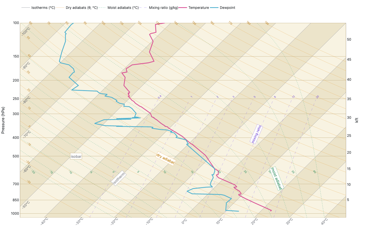
Skew-T log-P sounding
UWyo radiosonde OUN 72357, 00Z 2024-05-20
Example from the compendium of canonical charts
Python Code
"""Skew-T log-P sounding — UWyo radiosonde OUN 72357, 00Z 2024-05-20."""
import re
from pathlib import Path

# ── Palette + theme (matching the Plotly Studio gallery these charts ship in) ──
VIOLET, TEAL, GREEN, PINK, ORANGE = "#845EEE", "#52B3D0", "#55B685", "#DA5597", "#E9A23B"
PRIMARY, SECONDARY = VIOLET, TEAL
COLORWAY = [VIOLET, TEAL, GREEN, PINK, ORANGE]
BG, TEXT, GRID, MUTED = "#ffffff", "#1c2024", "#d9d9e0", "#60646c"
FONT = "Inter, -apple-system, BlinkMacSystemFont, sans-serif"
COLORSCALE = [[0, "rgba(132, 94, 238, 0.05)"], [1, "rgba(132, 94, 238, 0.9)"]]


def apply_theme(fig):
    """Light gallery theme: white background, Inter font, soft gridlines."""
    fig.update_layout(
        paper_bgcolor=BG, plot_bgcolor=BG, colorway=COLORWAY,
        font=dict(family=FONT, color=TEXT, size=12),
        legend=dict(font=dict(color=TEXT)),
        hoverlabel=dict(bgcolor="#f0f0f3", font=dict(color=TEXT, family=FONT), bordercolor=GRID),
    )
    fig.update_xaxes(gridcolor=GRID, linecolor=GRID, zerolinecolor=GRID)
    fig.update_yaxes(gridcolor=GRID, linecolor=GRID, zerolinecolor=GRID)


def fetch_csv(url, **kwargs):
    import io
    import pandas as pd
    import requests
    r = requests.get(url, timeout=60)
    r.raise_for_status()
    return pd.read_csv(io.StringIO(r.text), **kwargs)


def fetch_json(url):
    import requests
    r = requests.get(url, timeout=60)
    r.raise_for_status()
    return r.json()

import numpy as np
import pandas as pd
import plotly.graph_objects as go
from plotly.subplots import make_subplots

SKEW = 55   # skew factor in x-units per log10-pressure decade (~45° visual)

# Multiple data source attempts
UWYO_URL = (
    "https://weather.uwyo.edu/cgi-bin/sounding"
    "?region=naconf&TYPE=TEXT:LIST&YEAR=2024&MONTH=05&FROM=2000&TO=2000&STNM=72357"
)
# Iowa State University Mesonet radiosonde API (JSON)
IASTATE_URL = (
    "https://mesonet.agron.iastate.edu/json/raob.py"
    "?station=OUN&ts=2024051200"
)


def parse_uwyo_pre(text):
    m = re.search(r"<pre>(.*?)</pre>", text, re.DOTALL)
    if not m:
        return None
    lines = m.group(1).strip().split("\n")
    data_lines = [l for l in lines if re.match(r"\s*\d", l)]
    rows = []
    for l in data_lines:
        vals = l.split()
        if len(vals) >= 5:
            try:
                rows.append([float(v) for v in vals[:11]])
            except ValueError:
                pass
    if not rows:
        return None
    cols = ["PRES","HGHT","TEMP","DWPT","RELH","MIXR","DRCT","SKNT","THTA","THTE","THTV"]
    df = pd.DataFrame(rows, columns=cols[:len(rows[0])])
    return df[df["PRES"] > 0].dropna(subset=["PRES","TEMP","DWPT"])


def parse_iastate_json(data):
    """Parse Iowa State RAOB JSON response."""
    profiles = data.get("profiles", [])
    if not profiles:
        return None
    profile = profiles[0]
    levels  = profile.get("profile", [])
    rows = []
    for lv in levels:
        try:
            pres = float(lv.get("pres", 0))
            temp = float(lv.get("tmpc", 0))
            dwpt = float(lv.get("dwpc", 0))
            hght = float(lv.get("hght", 0))
            if pres > 0 and abs(temp) < 200 and abs(dwpt) < 200:
                rows.append({"PRES": pres, "TEMP": temp, "DWPT": dwpt, "HGHT": hght})
        except (ValueError, TypeError):
            pass
    if not rows:
        return None
    df = pd.DataFrame(rows)
    return df[df["PRES"] > 0].dropna(subset=["PRES","TEMP","DWPT"])


def synthetic_sounding():
    """Standard atmosphere + moist lapse rate sounding for demonstration."""
    import numpy as np
    pressures = [1013, 1000, 975, 950, 925, 900, 850, 800, 750, 700,
                 650, 600, 550, 500, 450, 400, 350, 300, 250, 200, 150, 100]
    rows = []
    T_sfc = 22.0   # surface temp °C
    Td_sfc = 14.0  # surface dewpoint °C
    for i, P in enumerate(pressures):
        # Dry lapse ~6.5°C/km, simplified with pressure
        k = np.log(1013 / P) / np.log(1013 / 100)
        T  = T_sfc - 60 * k
        Td = min(T, Td_sfc - 30 * k)
        rows.append({"PRES": float(P), "TEMP": T, "DWPT": Td, "HGHT": float(i * 500)})
    return pd.DataFrame(rows)


def fetch_sounding():
    import requests, warnings
    warnings.filterwarnings("ignore")
    requests.packages.urllib3.disable_warnings()

    for url, parser, label in [
        (UWYO_URL,    lambda t: parse_uwyo_pre(t),  "UWyo HTML"),
        (IASTATE_URL, lambda t: parse_iastate_json(__import__("json").loads(t)), "Iowa State JSON"),
    ]:
        try:
            r = requests.get(url, verify=False, timeout=20)
            if r.status_code == 200:
                df = parser(r.text)
                if df is not None and len(df) > 5:
                    print(f"  using {label}, {len(df)} levels")
                    return df, label
                print(f"  {label}: no usable data")
        except Exception as e:
            print(f"  {label} failed: {e}")

    print("  using synthetic standard-atmosphere sounding")
    return synthetic_sounding(), "Standard atmosphere (synthetic)"


# ── Thermodynamic constants ──────────────────────────────────────────────────
RD, CP, EPS, LV = 287.05, 1005.0, 0.622, 2.501e6   # J/kg/K, J/kg/K, –, J/kg
KAPPA = RD / CP                                     # ≈ 0.2854
P0 = 1000.0                                         # reference pressure (hPa)
P_BOT, P_TOP = 1050.0, 100.0                        # frame pressure limits
X_LEFT, X_RIGHT = -48.0, 45.0                       # frame temperature limits (skewed °C)

# Pressure levels labelled on the left axis (and drawn as horizontal isobars).
P_LABELS = [1000, 850, 700, 500, 400, 300, 250, 200, 150, 100]


def YP(P):
    """Vertical coordinate: log-pressure, 0 at 1000 hPa, increasing upward."""
    return np.log10(P0 / np.asarray(P, dtype=float))


def xskew(T_C, P):
    """Skew a temperature (°C) at pressure P into the diagram's x-coordinate."""
    return np.asarray(T_C, dtype=float) + SKEW * YP(P)


def es_hpa(T_C):
    """Saturation vapour pressure (hPa) — Bolton (1980)."""
    return 6.112 * np.exp(17.67 * T_C / (T_C + 243.5))


def sat_mixing_ratio(T_C, P):
    """Saturation mixing ratio (kg/kg) at temperature T_C (°C) and pressure P (hPa)."""
    e = es_hpa(T_C)
    return EPS * e / (P - e)


def family_trace(lines, color, name, width=0.8, dash=None):
    """Collapse a family of (value, cx, cy) lines into one trace. Families are labelled
    inline (rotated, in colour) rather than via the legend, so they stay off it."""
    xs, ys = [], []
    for _value, cx, cy in lines:
        xs.extend(list(cx) + [None])
        ys.extend(list(cy) + [None])
    return go.Scatter(x=xs, y=ys, mode="lines", name=name, showlegend=True,
                      hoverinfo="skip", line=dict(color=color, width=width, dash=dash))


def generate():
    print("fetching UWyo OUN 72357 radiosonde 00Z 2024-05-20 …")
    df, source = fetch_sounding()
    df = df[(df["PRES"] <= P_BOT) & (df["PRES"] >= P_TOP)].copy()

    # Hand-built Skew-T log-P, the way real sounding software (MetPy, SHARPpy) draws it:
    # a plain log-pressure y-axis with the temperature axis sheared ~45°, then the full
    # thermodynamic background drawn as line families — isotherms, isobars, dry adiabats,
    # moist (pseudo-)adiabats and mixing-ratio lines — over alternating shaded bands.
    Y_BOT, Y_TOP = float(YP(P_BOT)), float(YP(P_TOP))
    Pc = np.exp(np.linspace(np.log(P_BOT), np.log(P_TOP), 120))   # smooth pressure samples

    fig = go.Figure()

    # ── Background curve families ───────────────────────────────────────────────
    # Each family is a hand-drawn set of lines (one per "tick" value). We keep the
    # value with each line so we can label it like an axis tick further below.
    ISO_C  = "#9a9ca6"                  # isotherms
    DRY_C  = "rgba(233,162,59,0.55)"    # dry adiabats
    MOIST_C = "rgba(60,165,120,0.65)"   # moist adiabats
    MIX_C  = "rgba(132,94,238,0.60)"    # mixing-ratio lines

    # Isotherms: straight lines of constant T, sheared to the right (sampled over the
    # full pressure range so they can be labelled at any level, like the other families).
    isotherms = [(T, xskew(T, Pc), YP(Pc)) for T in range(-110, 51, 10)]
    fig.add_trace(family_trace(isotherms, ISO_C, "Isotherms (°C)", width=0.9))  # solid

    # Dry adiabats: constant potential temperature θ — T(P) = θ·(P/1000)^κ.
    dry = []
    for theta_C in range(-30, 200, 10):
        T_C = (theta_C + 273.15) * (Pc / P0) ** KAPPA - 273.15
        dry.append((theta_C, xskew(T_C, Pc), YP(Pc)))
    fig.add_trace(family_trace(dry, DRY_C, "Dry adiabats (θ, °C)", width=0.8))  # solid (source)

    # Moist (pseudo-)adiabats: integrate the saturated lapse rate upward from P_BOT.
    moist = []
    for T0_C in range(-20, 41, 5):
        T = T0_C + 273.15
        T_path = [T]
        for i in range(1, len(Pc)):
            dlnP = np.log(Pc[i]) - np.log(Pc[i - 1])
            ws = sat_mixing_ratio(T - 273.15, Pc[i - 1])
            dTdlnP = (RD * T + LV * ws) / (CP + (LV * LV * ws * EPS) / (RD * T * T))
            T = T + dTdlnP * dlnP
            T_path.append(T)
        moist.append((T0_C, xskew(np.array(T_path) - 273.15, Pc), YP(Pc)))
    fig.add_trace(family_trace(moist, MOIST_C, "Moist adiabats (°C)", width=0.9, dash="dot"))

    # Mixing-ratio lines: constant saturation mixing ratio w (dashed).
    mix_vals = [0.4, 1, 2, 3, 5, 8, 12, 20]   # g/kg
    mixing = []
    for w_gkg in mix_vals:
        w = w_gkg / 1000.0
        e = w * Pc / (EPS + w)                          # required vapour pressure
        T_C = 243.5 * np.log(e / 6.112) / (17.67 - np.log(e / 6.112))
        seg = Pc >= 250                                 # conventionally lower troposphere
        mixing.append((w_gkg, xskew(T_C[seg], Pc[seg]), YP(Pc[seg])))
    fig.add_trace(family_trace(mixing, MIX_C, "Mixing ratio (g/kg)", width=0.8, dash="dash"))  # dashed (source)

    # ── The sounding ────────────────────────────────────────────────────────────
    fig.add_trace(go.Scatter(
        x=xskew(df["TEMP"], df["PRES"]), y=YP(df["PRES"]),
        mode="lines", name="Temperature", line=dict(color=PINK, width=2.8),
        customdata=np.c_[df["TEMP"], df["PRES"]],
        hovertemplate="T = %{customdata[0]:.1f}°C @ %{customdata[1]:.0f} hPa<extra></extra>",
    ))
    fig.add_trace(go.Scatter(
        x=xskew(df["DWPT"], df["PRES"]), y=YP(df["PRES"]),
        mode="lines", name="Dewpoint", line=dict(color=TEAL, width=2.8),
        customdata=np.c_[df["DWPT"], df["PRES"]],
        hovertemplate="Td = %{customdata[0]:.1f}°C @ %{customdata[1]:.0f} hPa<extra></extra>",
    ))
    # ── Real height scale (km + kft) from the sounding's measured geopotential ───
    H = df["HGHT"].astype(float).values     # geopotential height, metres
    P = df["PRES"].astype(float).values
    order = np.argsort(H)
    Hs, Ps = H[order], P[order]

    def y_at_height(h_m):
        if h_m < Hs[0] or h_m > Hs[-1]:
            return None
        return float(YP(np.interp(h_m, Hs, Ps)))

    kft_ticks = [(h, y_at_height(h * 304.8)) for h in range(0, 56, 5)]
    kft_ticks = [(h, y) for h, y in kft_ticks if y is not None]

    # ── Frame: cream "paper" + alternating diagonal isotherm bands + isobars ────
    # Base paper fill.
    shapes = [dict(type="rect", xref="x", yref="y", layer="below",
                   x0=X_LEFT, x1=X_RIGHT, y0=Y_BOT, y1=Y_TOP,
                   line=dict(width=0), fillcolor="#f8f3e2")]
    # Every other 10 °C isotherm band, shaded as a skewed parallelogram (clipped to the
    # frame) so the alternating stripes run diagonally along the isotherms, not flat.
    for T in range(-110, 50, 10):
        if (T // 10) % 2 != 0:
            continue
        x0, x1 = T + SKEW * Y_BOT, (T + 10) + SKEW * Y_BOT
        x2, x3 = (T + 10) + SKEW * Y_TOP, T + SKEW * Y_TOP
        shapes.append(dict(type="path", xref="x", yref="y", layer="below",
                           path=f"M {x0},{Y_BOT} L {x1},{Y_BOT} L {x2},{Y_TOP} "
                                f"L {x3},{Y_TOP} Z",
                           fillcolor="rgba(206,186,140,0.28)", line=dict(width=0)))
    # Isobars (horizontal) drawn over the bands, then the frame border.
    shapes += [dict(type="line", xref="x", yref="y", layer="below",
                    x0=X_LEFT, x1=X_RIGHT, y0=YP(p), y1=YP(p),
                    line=dict(color="#cbb98f", width=1)) for p in P_LABELS]
    shapes.append(dict(type="rect", xref="x", yref="y", layer="below",
                       x0=X_LEFT, x1=X_RIGHT, y0=Y_BOT, y1=Y_TOP,
                       line=dict(color="#b29a63", width=1.2), fillcolor="rgba(0,0,0,0)"))

    # ── Tick labels for every hand-drawn family (each family is its own "axis") ──
    # Anchor a label where the line meets a frame edge ("top"/"bottom"), or where it
    # crosses a target pressure (a number, hPa) — inside the box.
    def line_anchor(cx, cy, where):
        xs, ys = np.asarray(cx, float), np.asarray(cy, float)
        if where == "top":
            idx = np.argsort(ys)[::-1]
        elif where == "bottom":
            idx = np.argsort(ys)
        elif where == "left":
            idx = np.argsort(xs)
        else:                                   # nearest a target pressure
            idx = np.argsort(np.abs(ys - float(YP(where))))
        for i in idx:
            if X_LEFT + 1.5 <= xs[i] <= X_RIGHT - 1.5 and Y_BOT <= ys[i] <= Y_TOP:
                return float(xs[i]), float(ys[i])
        return None

    annotations = []

    def label_family(lines, where, color, angle, fmt, dy=0, dx=0, edge_tol=None, size=9):
        for value, cx, cy in lines:
            anc = line_anchor(cx, cy, where)
            if anc is None:
                continue
            # Only label lines that actually reach the requested edge (avoids labelling
            # a line that merely clips a corner far from its edge).
            if edge_tol is not None:
                if where == "bottom" and anc[1] > Y_BOT + edge_tol:
                    continue
                if where == "top" and anc[1] < Y_TOP - edge_tol:
                    continue
            annotations.append(dict(
                x=anc[0], y=anc[1], xref="x", yref="y", text=fmt(value),
                showarrow=False, xshift=dx, yshift=dy, textangle=angle,
                font=dict(size=size, color=color)))

    # Isotherms (°C) labelled along the bottom (source convention); mixing ratio (g/kg)
    # at the top of each (250 hPa) line. Dry adiabats exit the left edge, so label there
    # (avoids colliding with the isotherm labels now on the bottom). Moist on the curve.
    label_family(isotherms, "bottom", MUTED, -45, lambda v: f"{v}°C", dy=-13, size=12)
    label_family(mixing, "top", "#7048d8", -45, lambda v: f"{v:g}", dy=10, dx=6)
    label_family(dry, "left", "#b97d1e", 45, lambda v: f"{v}", dx=8)
    label_family(moist, 600, "#2f8f63", 50, lambda v: f"{v}", dx=-9)

    # ── Inline family names, rotated to follow each line, in the family colour ───
    # Convert a data-space slope to the on-screen text angle for the 1280×800 export.
    PLOT_W, PLOT_H = 1280 - (70 + 70), 800 - (80 + 40)
    ppx = PLOT_W / (X_RIGHT - X_LEFT)
    ppy = PLOT_H / (Y_TOP - Y_BOT)

    def find_line(lines, value):
        return next(((v, cx, cy) for v, cx, cy in lines if v == value), None)

    def name_chip(x, y, text, line_color, line_width, text_color, angle=0.0, size=12, dx=0, dy=0):
        # A bordered "chip": the border uses the exact colour AND width of the family's
        # line, so it reads as a continuation of that reference line into the label.
        # The text uses a darker, readable shade. (Plotly borders can't be dashed.)
        annotations.append(dict(
            x=x, y=y, xref="x", yref="y", text=text, showarrow=False, textangle=angle,
            xshift=dx, yshift=dy, font=dict(size=size, color=text_color),
            bgcolor="rgba(255,255,255,0.94)", bordercolor=line_color,
            borderwidth=line_width, borderpad=3))

    def name_on_line(line, p_target, text, line_color, line_width, text_color,
                     size=12, dx=0, dy=0):
        if line is None:
            return
        _v, cx, cy = line
        xs, ys = np.asarray(cx, float), np.asarray(cy, float)
        i = int(np.argmin(np.abs(ys - float(YP(p_target)))))
        i0, i1 = max(i - 2, 0), min(i + 2, len(xs) - 1)
        ddx, ddy = xs[i1] - xs[i0], ys[i1] - ys[i0]
        angle = float(np.degrees(np.arctan2(-ddy * ppy, ddx * ppx)))
        angle = (angle + 90) % 180 - 90      # keep text upright (-90°…90°)
        if not (X_LEFT + 2 <= xs[i] <= X_RIGHT - 2):
            return
        name_chip(float(xs[i]), float(ys[i]), text, line_color, line_width, text_color,
                  angle, size, dx, dy)

    # Each chip's border = its family line's exact (colour, width); text = readable shade.
    name_on_line(find_line(dry, 30), 520, "dry adiabat", DRY_C, 0.8, "#c5881f", size=13)
    # Moist adiabat & mixing ratio: lifted above their lines (+dy), in the clear wedge
    # to the right of the sounding so they don't sit on the temperature/dewpoint traces.
    name_on_line(find_line(moist, 30), 680, "moist adiabat", MOIST_C, 0.9, "#2f8f63", size=13, dy=11)
    name_on_line(find_line(mixing, 8), 400, "mixing ratio", MIX_C, 0.8, "#7048d8", size=12, dy=11)
    name_on_line(find_line(isotherms, -30), 650, "isotherm", ISO_C, 0.9, "#787b85", size=13)
    # Isobars are horizontal lines (drawn as shapes): a flat chip on the 500 hPa line.
    name_chip(X_LEFT + 16, float(YP(500)), "isobar", "#cbb98f", 1.0, "#787b85", angle=0, size=13)

    # Dummy trace so the overlaying right-hand height axis (kft) renders.
    fig.add_trace(go.Scatter(x=[X_LEFT], y=[Y_BOT], xaxis="x", yaxis="y2",
                             mode="markers", marker=dict(opacity=0),
                             showlegend=False, hoverinfo="skip"))

    fig.update_layout(
        title=dict(text=f"Skew-T log-P — OUN Norman OK ({source})", x=0.5),
        shapes=shapes,
        annotations=annotations,
        xaxis=dict(visible=False, showgrid=False, zeroline=False,
                   range=[X_LEFT, X_RIGHT], autorange=False, fixedrange=True),
        yaxis=dict(title=dict(text="Pressure (hPa)"), tickmode="array",
                   tickvals=[float(YP(p)) for p in P_LABELS],
                   ticktext=[str(p) for p in P_LABELS],
                   range=[Y_BOT, Y_TOP], autorange=False,
                   showgrid=False, zeroline=False, side="left"),
        # Right height scale in thousands of feet, from the measured geopotential.
        yaxis2=dict(title=dict(text="kft"), tickmode="array",
                    tickvals=[y for _, y in kft_ticks],
                    ticktext=[str(h) for h, _ in kft_ticks],
                    range=[Y_BOT, Y_TOP], autorange=False,
                    overlaying="y", side="right", showgrid=False, zeroline=False),
        legend=dict(orientation="h", y=1.10),
        margin=dict(t=80, b=40, l=70, r=70),
        height=640,
    )
    apply_theme(fig)
    return fig


fig = generate()
fig.show()
Made with Plotly