
Seismic envelope, waveform & spectrogram
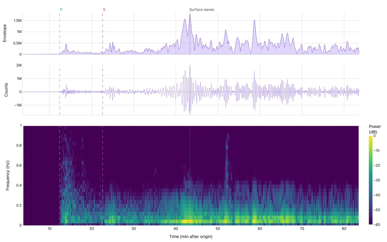
M9.1 Tōhoku at IU.ANMO
Example from the compendium of canonical charts
Python Code
"""Seismic envelope, waveform & spectrogram — M9.1 Tōhoku at IU.ANMO.

The canonical way a seismologist looks at a single station's record of a distant
earthquake: the broadband envelope on top (where the energy is), the raw
waveform in the middle (the wiggles), and a spectrogram underneath (how the
frequency content evolves as the P, S, and surface waves sweep through).

Real data: the M9.1 Tōhoku earthquake of 2011-03-11 (origin 05:46:24 UTC),
recorded on the vertical broadband channel (BHZ) of station IU.ANMO in
Albuquerque, New Mexico — ~84° away — fetched as ASCII from the IRIS FDSN
timeseries web service.
"""
from pathlib import Path

# ── Palette + theme (matching the Plotly Studio gallery these charts ship in) ──
VIOLET, TEAL, GREEN, PINK, ORANGE = "#845EEE", "#52B3D0", "#55B685", "#DA5597", "#E9A23B"
PRIMARY, SECONDARY = VIOLET, TEAL
COLORWAY = [VIOLET, TEAL, GREEN, PINK, ORANGE]
BG, TEXT, GRID, MUTED = "#ffffff", "#1c2024", "#d9d9e0", "#60646c"
FONT = "Inter, -apple-system, BlinkMacSystemFont, sans-serif"
COLORSCALE = [[0, "rgba(132, 94, 238, 0.05)"], [1, "rgba(132, 94, 238, 0.9)"]]


def apply_theme(fig):
    """Light gallery theme: white background, Inter font, soft gridlines."""
    fig.update_layout(
        paper_bgcolor=BG, plot_bgcolor=BG, colorway=COLORWAY,
        font=dict(family=FONT, color=TEXT, size=12),
        legend=dict(font=dict(color=TEXT)),
        hoverlabel=dict(bgcolor="#f0f0f3", font=dict(color=TEXT, family=FONT), bordercolor=GRID),
    )
    fig.update_xaxes(gridcolor=GRID, linecolor=GRID, zerolinecolor=GRID)
    fig.update_yaxes(gridcolor=GRID, linecolor=GRID, zerolinecolor=GRID)


def fetch_csv(url, **kwargs):
    import io
    import pandas as pd
    import requests
    r = requests.get(url, timeout=60)
    r.raise_for_status()
    return pd.read_csv(io.StringIO(r.text), **kwargs)


def fetch_json(url):
    import requests
    r = requests.get(url, timeout=60)
    r.raise_for_status()
    return r.json()

import numpy as np
import plotly.graph_objects as go
from plotly.subplots import make_subplots


# IU.ANMO vertical broadband, 80-minute window covering P, S and the big
# Rayleigh-wave package. The segment starts 3.60 min after the origin time.
URL = (
    "https://service.iris.edu/irisws/timeseries/1/query?"
    "net=IU&sta=ANMO&loc=00&cha=BHZ"
    "&starttime=2011-03-11T05:50:00&endtime=2011-03-11T07:10:00"
    "&format=ascii&output=ascii"
)
FS = 20.0                 # BHZ sample rate (sps)
ORIGIN_OFFSET = 3.60      # window start, in minutes after the 05:46:24 origin

# Approximate teleseismic arrival times at ~84° (IASP91), in minutes after origin.
T_P = 12.4
T_S = 22.6


def _parse_ascii(text):
    """Parse an IRIS TSPAIR ASCII payload into a 1-D sample array."""
    vals = []
    for line in text.splitlines():
        line = line.strip()
        if not line or line.upper().startswith(("TIMESERIES", "#")):
            continue
        parts = line.split()
        try:
            vals.append(float(parts[-1]))
        except (ValueError, IndexError):
            continue
    return np.asarray(vals, dtype=float)


def _synthetic():
    """Fallback teleseism: noise floor + P, S and a dominant surface-wave train."""
    rng = np.random.default_rng(11)
    n = int(80 * 60 * FS)
    t = np.arange(n) / FS / 60 + ORIGIN_OFFSET   # minutes since origin
    x = rng.normal(0, 1.0, n)

    def packet(t0, dur, freq, amp):
        tt = t - t0
        m = tt >= 0
        env = np.zeros_like(t)
        env[m] = np.exp(-tt[m] / dur) * (1 - np.exp(-tt[m] / (dur * 0.05)))
        return amp * env * np.sin(2 * np.pi * freq * (t - t0) * 60)

    x += packet(T_P, 2.5, 1.2, 6)      # P: short, higher frequency
    x += packet(T_S, 4.0, 0.6, 14)     # S: stronger, lower frequency
    x += packet(43.0, 9.0, 0.04, 90)   # Rayleigh surface waves: dominant, very low freq
    return x


def _load():
    import requests
    try:
        r = requests.get(URL, verify=False, timeout=60)
        r.raise_for_status()
        x = _parse_ascii(r.text)
        if len(x) < 10000:
            raise ValueError(f"too few samples: {len(x)}")
        print(f"  fetched {len(x)} samples ({len(x)/FS/60:.0f} min) from IRIS")
        return x, False
    except Exception as e:  # noqa: BLE001 — data-prep tool, degrade gracefully
        print(f"  IRIS fetch failed ({e}); using synthetic teleseism")
        return _synthetic(), True


def generate():
    print("fetching seismic waveform …")
    from scipy import signal

    raw, synthetic = _load()

    # ── Pre-process: demean, then band-pass to the teleseismic band ───────────
    x = raw - raw.mean()
    b, a = signal.butter(4, [0.02, 5.0], btype="bandpass", fs=FS)
    xf = signal.filtfilt(b, a, x)

    n = len(xf)
    t_min = np.arange(n) / FS / 60 + ORIGIN_OFFSET   # minutes since origin

    # ── Envelope (analytic-signal amplitude), smoothed for display ────────────
    env = np.abs(signal.hilbert(xf))
    win = int(10 * FS)                                # 10-second smoothing
    env = np.convolve(env, np.ones(win) / win, mode="same")

    # ── Spectrogram (STFT) on the full-rate band-passed trace ─────────────────
    f, t_spec, Sxx = signal.spectrogram(
        xf, fs=FS, nperseg=512, noverlap=384, scaling="spectrum"
    )
    fmask = f <= 1.0
    f, Sxx = f[fmask], Sxx[fmask]
    Z = 10 * np.log10(Sxx + 1e-12)                    # power in dB
    Z = Z - Z.max()                                   # reference to peak (0 dB)
    t_spec = t_spec / 60 + ORIGIN_OFFSET
    # Thin the time axis and round to keep the interactive JSON compact
    stride = max(1, Z.shape[1] // 400)
    t_spec, Z = t_spec[::stride], np.round(Z[:, ::stride]).astype(int)

    # ── Decimate waveform + envelope for plotting (display only) ──────────────
    dec = 20
    tw = t_min[::dec]
    wave = signal.decimate(xf, dec, ftype="fir")
    envd = env[::dec][: len(wave)]
    tw = tw[: len(wave)]

    # ── Three stacked panels sharing the time axis ────────────────────────────
    fig = make_subplots(
        rows=3, cols=1, shared_xaxes=True, vertical_spacing=0.05,
        row_heights=[0.22, 0.26, 0.52],
    )

    fig.add_trace(go.Scatter(
        x=tw, y=envd, mode="lines", line=dict(color=VIOLET, width=1),
        fill="tozeroy", fillcolor="rgba(132, 94, 238, 0.25)",
        hovertemplate="t=%{x:.1f} min<br>env=%{y:.0f}<extra></extra>",
    ), row=1, col=1)

    fig.add_trace(go.Scatter(
        x=tw, y=wave, mode="lines", line=dict(color=VIOLET, width=0.6),
        hovertemplate="t=%{x:.1f} min<br>amp=%{y:.0f}<extra></extra>",
    ), row=2, col=1)

    fig.add_trace(go.Heatmap(
        x=t_spec, y=f, z=Z,
        colorscale="Viridis", zmin=-60, zmax=0,
        colorbar=dict(title="Power<br>(dB)", thickness=12, len=0.5, y=0.24,
                      yanchor="middle"),
        hovertemplate="t=%{x:.1f} min<br>f=%{y:.2f} Hz<br>%{z:.0f} dB<extra></extra>",
    ), row=3, col=1)

    # ── Mark the P, S and surface-wave arrivals across all panels ─────────────
    for tt, color in ((T_P, TEAL), (T_S, PINK)):
        fig.add_vline(x=tt, line=dict(color=color, width=1.2, dash="dash"))
    peak_min = float(tw[np.argmax(envd)])
    fig.add_vline(x=peak_min, line=dict(color=MUTED, width=1.2, dash="dot"))

    fig.add_annotation(x=T_P, y=1.0, yref="paper", text="P", showarrow=False,
                       font=dict(color=TEAL, size=12), xanchor="left", yanchor="bottom")
    fig.add_annotation(x=T_S, y=1.0, yref="paper", text="S", showarrow=False,
                       font=dict(color=PINK, size=12), xanchor="left", yanchor="bottom")
    fig.add_annotation(x=peak_min, y=1.0, yref="paper", text="Surface waves",
                       showarrow=False, font=dict(color=MUTED, size=12),
                       xanchor="left", yanchor="bottom")

    fig.update_yaxes(title_text="Envelope", row=1, col=1)
    fig.update_yaxes(title_text="Counts", row=2, col=1)
    fig.update_yaxes(title_text="Frequency (Hz)", range=[0, 1], row=3, col=1)
    fig.update_xaxes(title_text="Time (min after origin)", row=3, col=1)

    fig.update_layout(
        margin=dict(t=40, b=55, l=75, r=80),
        height=560,
        showlegend=False,
    )

    apply_theme(fig)
    return fig


fig = generate()
fig.show()
Made with Plotly