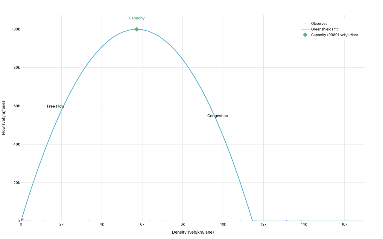
Traffic Fundamental Diagram

Python Code

"""Transportation — Traffic Fundamental Diagram (flow vs. density)."""


import numpy as np
import plotly.graph_objects as go


def generate():
    url = (
        "https://raw.githubusercontent.com/TrafficGCN/"
        "mfd_traffic_congestion_for_data_scientists/main/data/"
        "eth_bolton_sensor_data_utd19.csv"
    )
    try:
        df = fetch_csv(url)
        print(f"  loaded {len(df)} rows, cols: {list(df.columns)}")

        # Filter out error rows — ERROR==1 means flagged; NaN means clean
        if "ERROR" in df.columns:
            df = df[df["ERROR"].isna() | (df["ERROR"] == 0)].copy()

        # Drop extreme outliers in density (sensor glitches)
        density_95 = df["DENSITY"].quantile(0.995)
        df = df[df["DENSITY"] <= density_95].copy()

        # Pick detector with most data
        id_col = "ID"
        best_id = df[id_col].value_counts().idxmax()
        df = df[df[id_col] == best_id].copy()
        print(f"  detector {best_id}: {len(df)} clean rows")

        density = df["DENSITY"].values
        flow = df["FLOW"].values

    except Exception as e:
        print(f"  data fetch failed ({e}), generating synthetic data")
        # Greenshields fundamental diagram: q = vf * k * (1 - k/kj)
        rng = np.random.default_rng(42)
        vf = 100.0      # free-flow speed (km/h)
        kj = 150.0      # jam density (veh/km/lane)
        density_raw = rng.uniform(0, kj, 3000)
        flow_ideal = vf * density_raw * (1 - density_raw / kj)
        noise = rng.normal(0, flow_ideal.max() * 0.06, len(density_raw))
        flow_raw = np.clip(flow_ideal + noise, 0, None)
        # scatter around capacity region
        density = density_raw
        flow = flow_raw

    # Greenshields model fit
    k = np.linspace(0, density.max() * 1.05, 300)
    # Fit vf and kj via linear regression on v = vf*(1-k/kj) → v = vf - (vf/kj)*k
    valid = density > 1
    speed = flow[valid] / density[valid]
    coeffs = np.polyfit(density[valid], speed, 1)   # speed = m*k + b
    vf_fit = coeffs[1]
    kj_fit = -vf_fit / coeffs[0] if coeffs[0] != 0 else density.max()
    q_fit = vf_fit * k * (1 - k / kj_fit)
    q_fit = np.clip(q_fit, 0, None)

    # Capacity point
    k_cap = kj_fit / 2
    q_cap = vf_fit * k_cap * (1 - k_cap / kj_fit)

    fig = go.Figure()

    # Scatter of observed data
    fig.add_trace(go.Scattergl(
        x=density,
        y=flow,
        mode="markers",
        marker=dict(size=3, opacity=0.4, color=VIOLET),
        name="Observed",
        hovertemplate="Density: %{x:.1f} veh/km/lane<br>Flow: %{y:.0f} veh/hr/lane<extra></extra>",
    ))

    # Greenshields fit
    fig.add_trace(go.Scatter(
        x=k,
        y=q_fit,
        mode="lines",
        line=dict(color=TEAL, width=2.5),
        name="Greenshields fit",
        hovertemplate="k=%{x:.1f}<br>q=%{y:.0f}<extra></extra>",
    ))

    # Capacity point
    fig.add_trace(go.Scatter(
        x=[k_cap],
        y=[q_cap],
        mode="markers",
        marker=dict(size=12, color=GREEN, symbol="diamond"),
        name=f"Capacity ({q_cap:.0f} veh/hr/lane)",
        hovertemplate="Capacity<br>k=%{x:.1f}<br>q=%{y:.0f}<extra></extra>",
    ))

    # Annotations for zones
    x_range = density.max()
    fig.add_annotation(
        x=k_cap * 0.3, y=q_cap * 0.6,
        text="Free Flow",
        showarrow=False,
        font=dict(size=13, color=TEXT),
        xanchor="center",
    )
    fig.add_annotation(
        x=k_cap, y=q_cap * 1.06,
        text="Capacity",
        showarrow=False,
        font=dict(size=13, color=GREEN),
        xanchor="center",
    )
    fig.add_annotation(
        x=min(k_cap * 1.7, x_range * 0.85), y=q_cap * 0.55,
        text="Congestion",
        showarrow=False,
        font=dict(size=13, color=TEXT),
        xanchor="center",
    )

    fig.update_layout(
        xaxis=dict(title="Density (veh/km/lane)", rangemode="tozero"),
        yaxis=dict(title="Flow (veh/hr/lane)", rangemode="tozero"),
        legend=dict(x=0.98, y=0.98, xanchor="right", yanchor="top"),
        margin=dict(t=50, b=60, l=70, r=60),
    )

    return fig


if __name__ == "__main__":
    generate()

Made with Plotly