
City trees
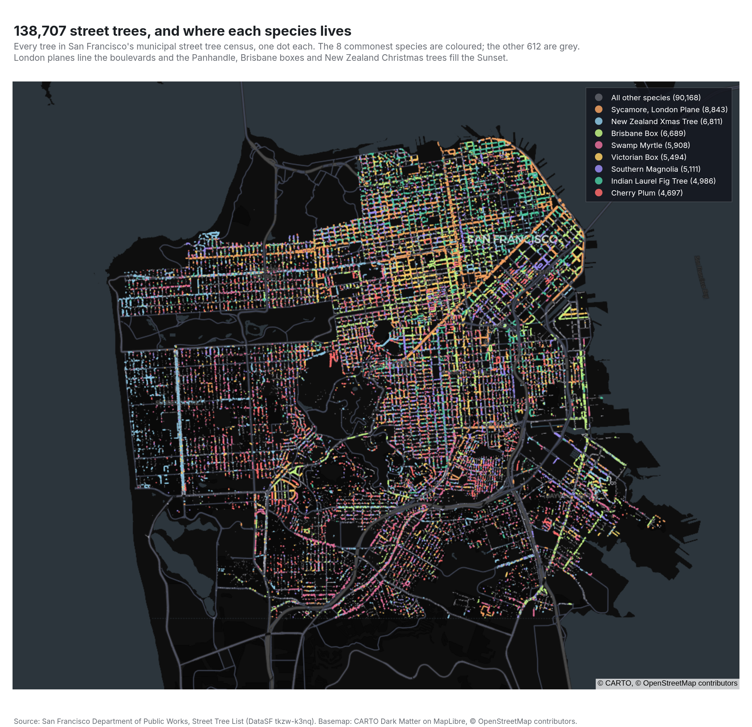
every street tree in San Francisco, coloured by species
Example from Plotly for highly customizable print-ready data visualization · shared helpers
Python Code
"""City trees — every street tree in San Francisco, coloured by species.

A city-scale MapLibre map with the new token-free `map` trace: 139,000
points from the municipal tree census, the eight commonest species in
colour and the rest in grey, drawn small enough that the streets emerge
from the trees themselves, over a dark basemap whose own labels name the
neighbourhoods.
"""
from pathlib import Path

from _shared import fetch_csv, save, base_layout, titles, INK, MUTED, hex_to_rgba

import numpy as np
import pandas as pd
import plotly.graph_objects as go

CHART_NUM = 30
URL = "https://data.sfgov.org/api/views/tkzw-k3nq/rows.csv?accessType=DOWNLOAD"
TOP = 8
# A categorical palette that reads on a dark basemap.
PALETTE = ["#f4a261", "#8ecae6", "#c3f584", "#e76f9b", "#ffd166", "#9b8cf5", "#4cc9a0", "#ff6b6b"]


def generate():
    df = fetch_csv(URL, usecols=["species", "latitude", "longitude", "mapdbh"], low_memory=False).dropna(subset=["latitude", "longitude"])
    df = df[df["latitude"].between(37.70, 37.83) & df["longitude"].between(-122.52, -122.35)]
    df["common"] = df["species"].str.split(" :: ").str[-1].str.replace(r" '.*'$", "", regex=True)
    top = df["common"].value_counts().head(TOP)
    fig = go.Figure()
    rest = df[~df["common"].isin(top.index)]
    fig.add_trace(go.Scattermap(lat=rest["latitude"], lon=rest["longitude"], mode="markers", name=f"All other species ({len(rest):,})",
                                marker=dict(size=2.2, color="rgba(200,200,210,0.35)"), hoverinfo="skip"))
    for (name, n), color in zip(top.items(), PALETTE):
        g = df[df["common"] == name]
        fig.add_trace(go.Scattermap(lat=g["latitude"], lon=g["longitude"], mode="markers", name=f"{name} ({n:,})",
                                    marker=dict(size=3.2, color=color, opacity=0.85),
                                    hovertemplate="%{customdata[0]}<br>trunk %{customdata[1]:.0f} in<extra></extra>",
                                    customdata=np.c_[g["species"], g["mapdbh"].fillna(0)]))
    fig.update_layout(**base_layout(margin=dict(l=20, r=20, t=130, b=60), showlegend=True,
                                    legend=dict(x=0.99, y=0.99, xanchor="right", yanchor="top", bgcolor="rgba(20,22,30,0.85)",
                                                font=dict(size=12, color="white"), itemsizing="constant", bordercolor="rgba(255,255,255,0.15)", borderwidth=1)))
    fig.update_layout(map=dict(style="carto-darkmatter", center=dict(lat=37.757, lon=-122.443), zoom=12.05, bearing=0, pitch=0),
                      map_domain=dict(x=[0, 1], y=[0, 1]))
    titles(fig, f"{len(df):,} street trees, and where each species lives",
           f"Every tree in San Francisco's municipal street tree census, one dot each. The {TOP} commonest species are coloured; the other {df['common'].nunique() - TOP:,} are grey.<br>"
           "London planes line the boulevards and the Panhandle, Brisbane boxes and New Zealand Christmas trees fill the Sunset.",
           "Source: San Francisco Department of Public Works, Street Tree List (DataSF tkzw-k3nq). Basemap: CARTO Dark Matter on MapLibre, © OpenStreetMap contributors.", lift=18)
    save(CHART_NUM, fig, width=1200, height=1160)
Made with Plotly