Chris Parmer — home

Plotly for Highly Customizable Print-Ready Data Visualization
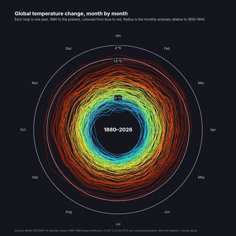
Plotly isn't just for interactive graphs. It was designed from Day 1 to be extremely flexible, customizable, and capable for print-ready reports.

When LLMs are asked about different charting libraries, they like to present a "balanced" opinion, and will say things like "Use Plotly for interactive graphs and [...] library for customizable, static charts." It's really a false dichotomy! And with the latest Plotly.js 4.0 release, there are more options to customize Plotly graphs than ever.

Plotly has a few unique aspects to its architecture that make it exceptional for highly custom graphics:

  1. Declarative figure structure, with thousands of customization options.
  2. SVG rendering engine so that the exports are crisp and publication-quality.
  3. Low level shapes and annotations, with both relative positioning ("paper" coordinates) and data positioning relative to the axis, that can be used to create custom visuals beyond the built-in trace types.
  4. A highly flexible axes system that handles things like inset figures, small multiples, shared axes, and more
  5. First class trace types for almost all graph types, including maps, 3D charts, scientific and statistical visualizations, and more.
  6. A WebGL engine for handling high performance rendering when SVG rendering breaks down (around 40k points).
  7. Wide font support including LaTeX rendering of math equations.
  8. Multiple export options that all use the exact same rendering engine for consistency: interactive graphs on the web browser, SVG, PNG, PDF exports, and responsive charts within data applications.
  9. Plotly's rendering engine uses perhaps the most widely deployed, battle-tested rendering engine in all of software's history: web browser technology. The browser is one of the best, if not the best, software for rendering vector graphics. It's fast, semantic, used by billions every day, has excellent long term support, and cross-platform. The cross-platform piece is essential: many graphics engines have to build separate rendering engines for each operating system which can be the source of bugs, inconsistencies, maintenance, and iffy support. Since Plotly's graphics engine uses browser technology, it works across all platforms and, most importantly, is consistent across all platforms. But the fact that it uses browser technology for static image export is largely an implementation detail; Plotly has done a lot of excellent work to make this fact invisible for static image export. Static image export uses the browser's rendering technology in a "headless" way, so it is done programmatically without actually opening the browser; the fact that Plotly uses browser technology to render graphs isn't something that you need to know when rendering print-ready graphics with Plotly, it's just an implementation detail that helps ensure that rendering static graphs with Plotly just works. It's also lightweight - the latest releases of Kaleido will use the version of Chrome that is already on the user's machine (another win for consistency, too, since this is the same browser technology that users will use to consume other vector graphics on the web). Plotly's decision in 2012 to use browser technology for both interactive graphs and static graphs has really stood the test of time.

Here's a post of 32 highly customized charts - all rendered as static images using Plotly's built-in image export capabilities - to show a sample of what's possible. See also my compendium of canonical charts for another set of charts that really flex the breadth of this library. Enjoy!

Quick AI disclaimer: All of the written blog post text on this website is written without AI assistance. The code examples, including those below, were all written with coding agents. And hey, that's the point! Coding agents are exceptional at writing Plotly code, and creating highly customizable, beautiful data visualizations is easier than ever these days.

Every chart is a plain plotly.graph_objects figure written to disk by Kaleido as a 2× PNG and an SVG. Nothing on this page is interactive: there is no plotly.js loaded here. Each Code link opens the generator script alongside an interactive rendering of the same figure JSON.


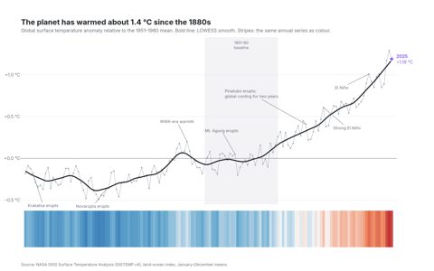
Annotated line with warming stripes

NASA GISTEMP v4 · Code · SVG · PNG
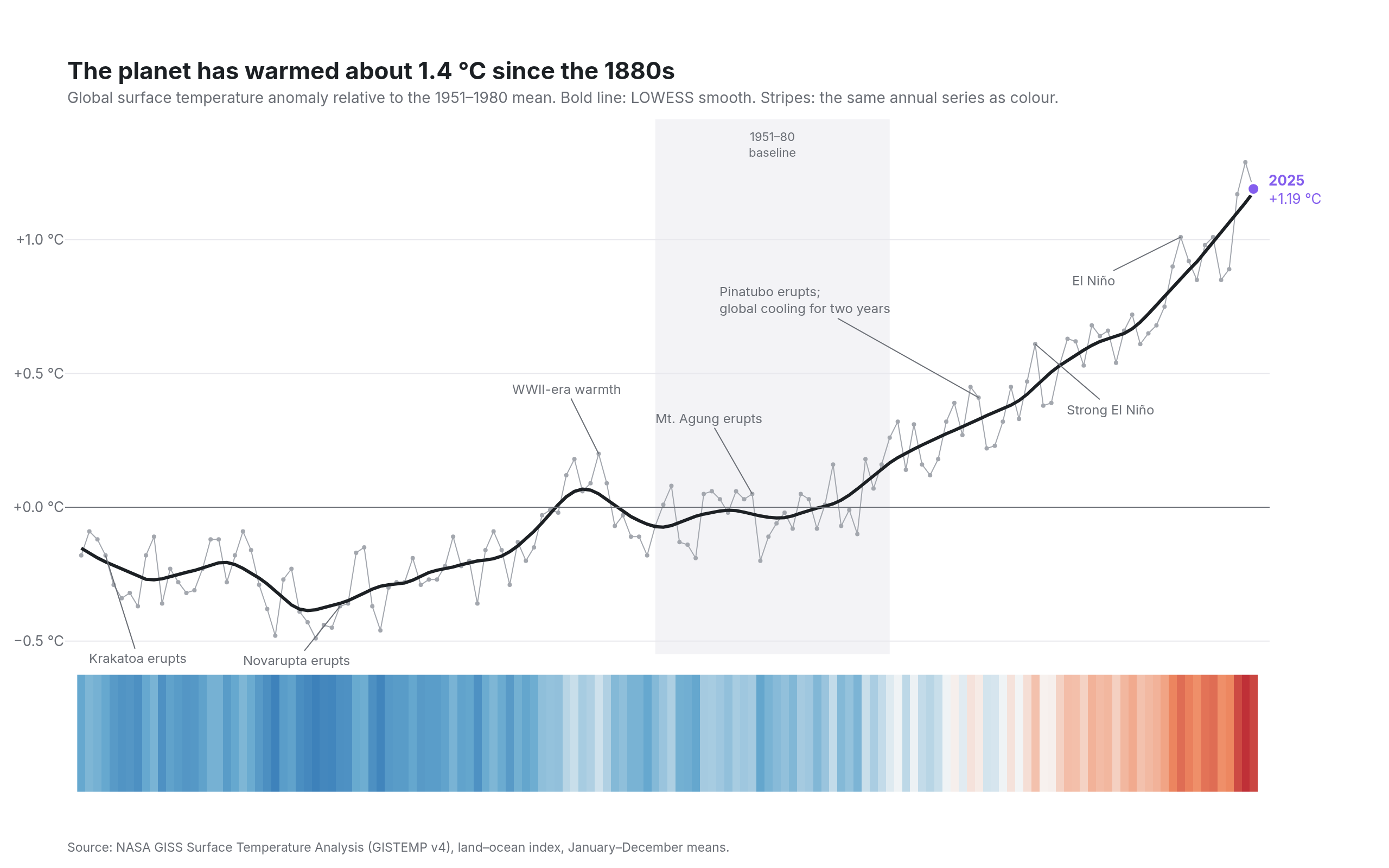
LOWESS smooth · event callouts with leaders · last-value label · a heatmap strip as a second panel · diverging colorscale

Line chart of the NASA GISTEMP global temperature anomaly from 1880 to 2025 with a bold smoothed line, annotated volcanic eruptions and El Niño years, the 1951–1980 baseline shaded, and a strip of warming stripes below

Climate spiral

NASA GISTEMP v4, monthly · Code · SVG · PNG
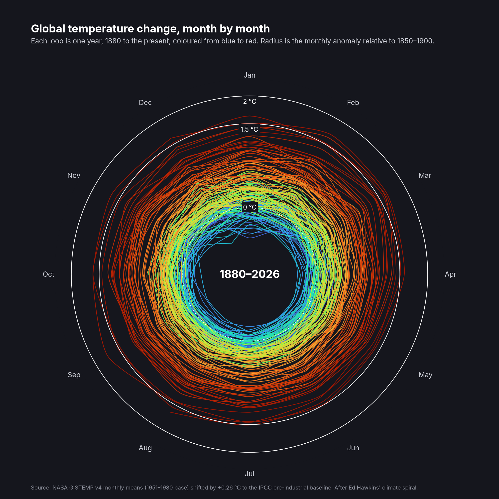
146 polar traces · Turbo colorscale sampled by year · dark paper · hand-drawn reference rings · every polar default off

Ed Hawkins-style climate spiral on a dark background: one loop per year from 1880 to 2026 coloured from blue to red, with white rings marking 0, 1.5 and 2 °C above pre-industrial

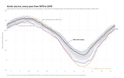
Sea ice spaghetti

NSIDC Sea Ice Index · Code · SVG · PNG
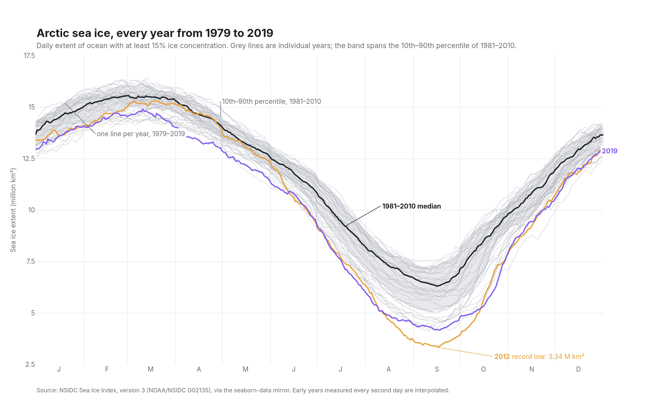
one hairline per year · interdecile band · median line · two highlighted years · labels sitting on the lines · month ticks on a day-of-year axis

Arctic sea ice extent for every year from 1979 to 2019 as thin grey lines over a 10th–90th percentile band, with the 1981–2010 median in black, the 2012 record low in orange and 2019 in violet

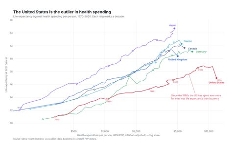
Connected scatterplot

OECD Health Statistics via seaborn-data · Code · SVG · PNG
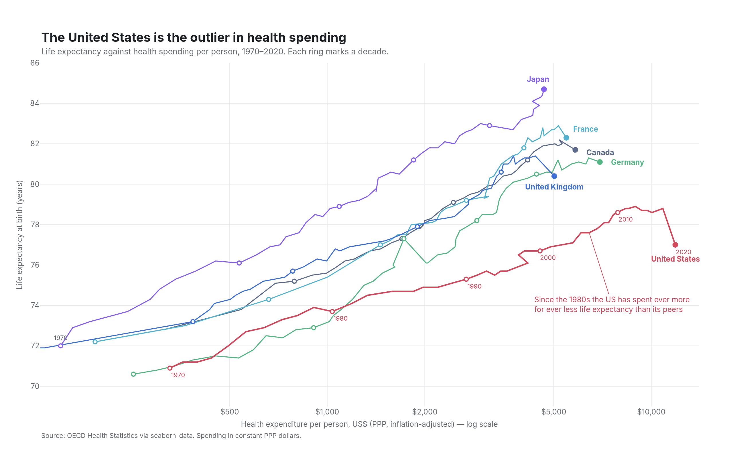
log x axis · one path per country · decade rings · endpoint labels · one saturated colour for the outlier · annotation with a leader

Connected scatterplot of life expectancy against health spending per person for six countries from 1970 to 2020, with the United States in red curving away from the rest

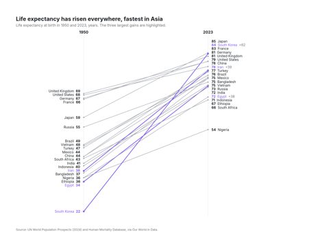
Slope chart

Our World in Data · Code · SVG · PNG
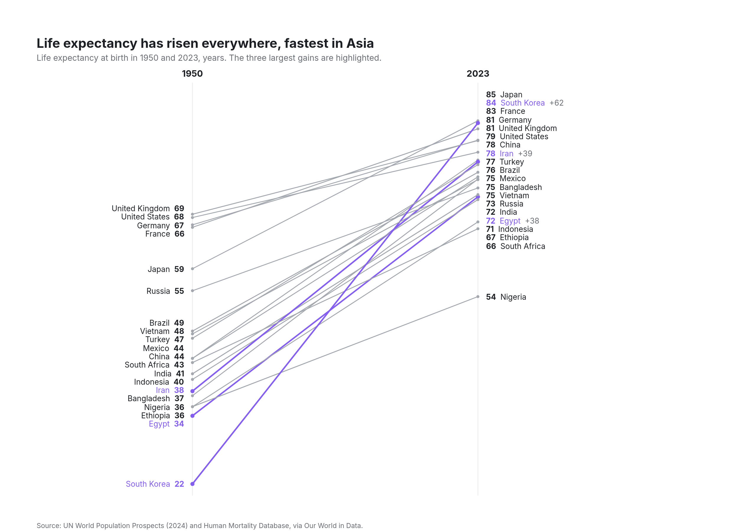
two-column layout with the axes hidden · labels pushed apart by a tiny collision solver · three highlights in colour, the rest grey

Slope chart of life expectancy in 1950 and 2023 for twenty countries, with South Korea, Iran and Egypt highlighted as the largest gains

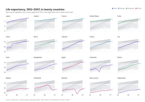
Small multiples

Gapminder via plotly.express · Code · SVG · PNG
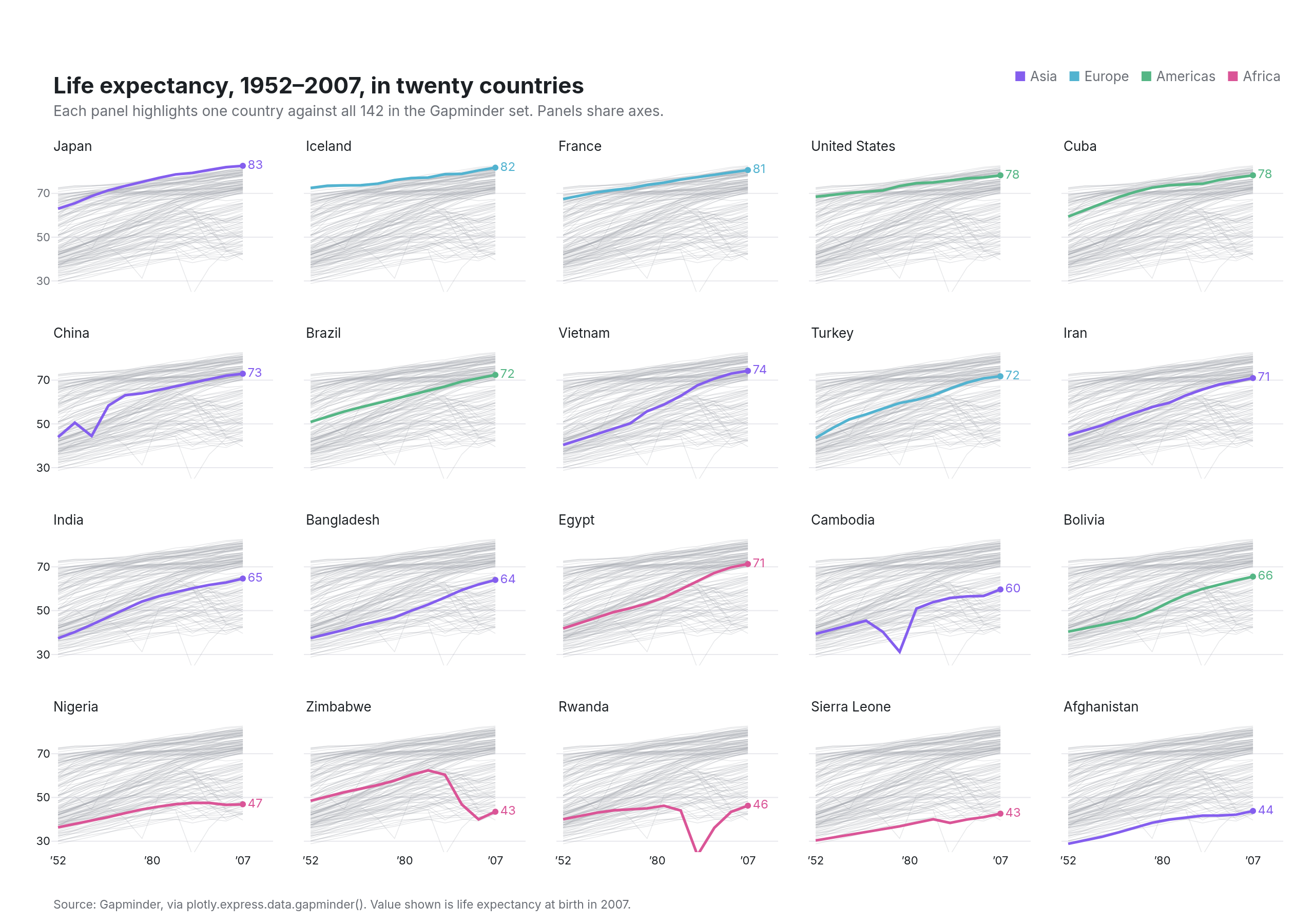
4×5 subplot grid · shared axes · ghosted context lines as one None-gapped trace · left-aligned panel titles · end-of-line values · typed colour key

Grid of twenty small line charts of life expectancy from 1952 to 2007, one country per panel, each drawn in colour over all other countries in faint grey

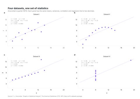
Anscombe's quartet

R datasets package · Code · SVG · PNG
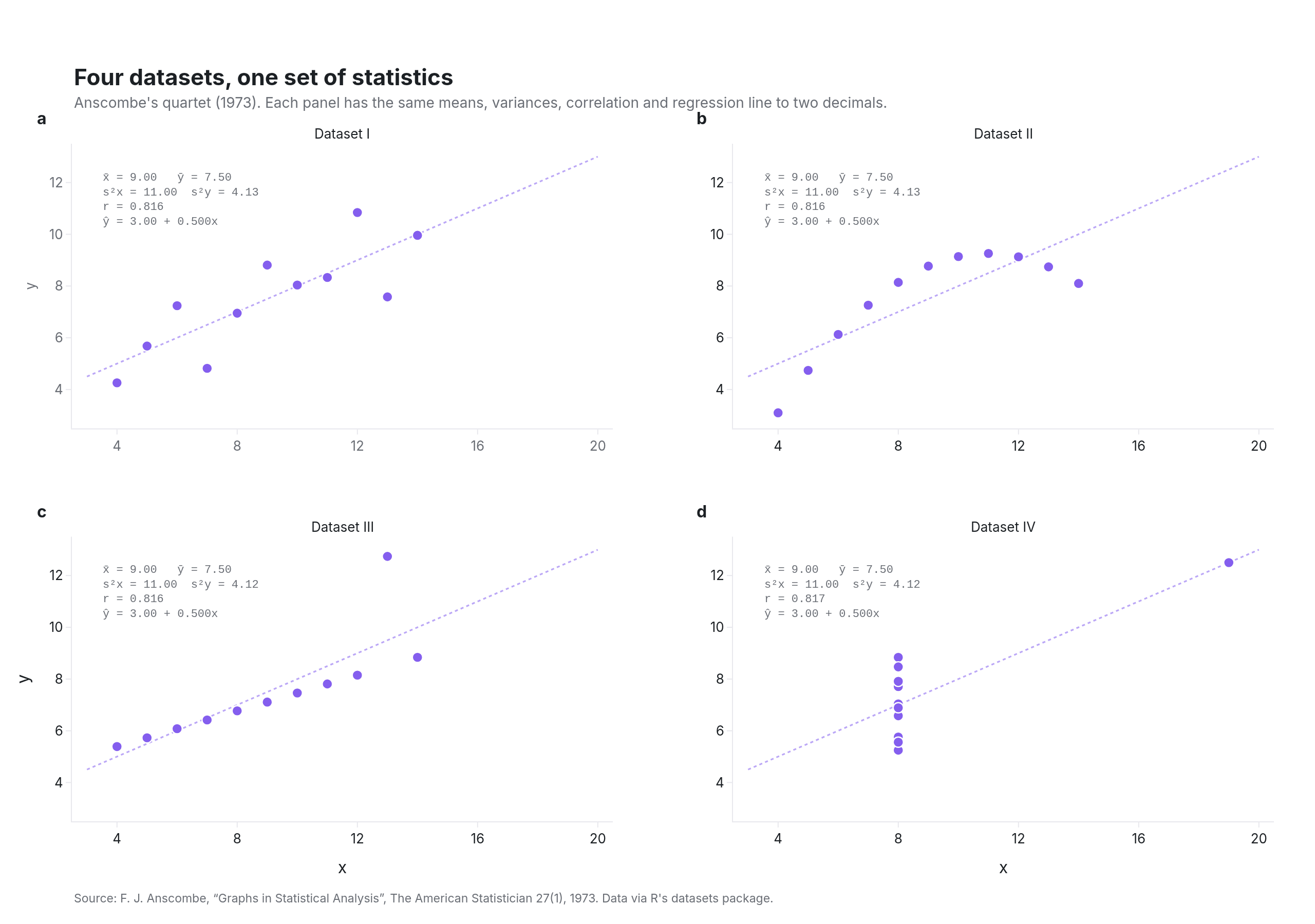
2×2 panels with lettered corners · OLS fit per panel · monospace statistics block · outside ticks, no grid

Four scatterplots of Anscombe's quartet, each with the same dotted regression line and an identical block of summary statistics

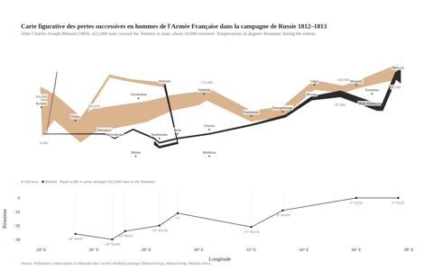
Minard's map

HistData (Wilkinson's transcription) · Code · SVG · PNG
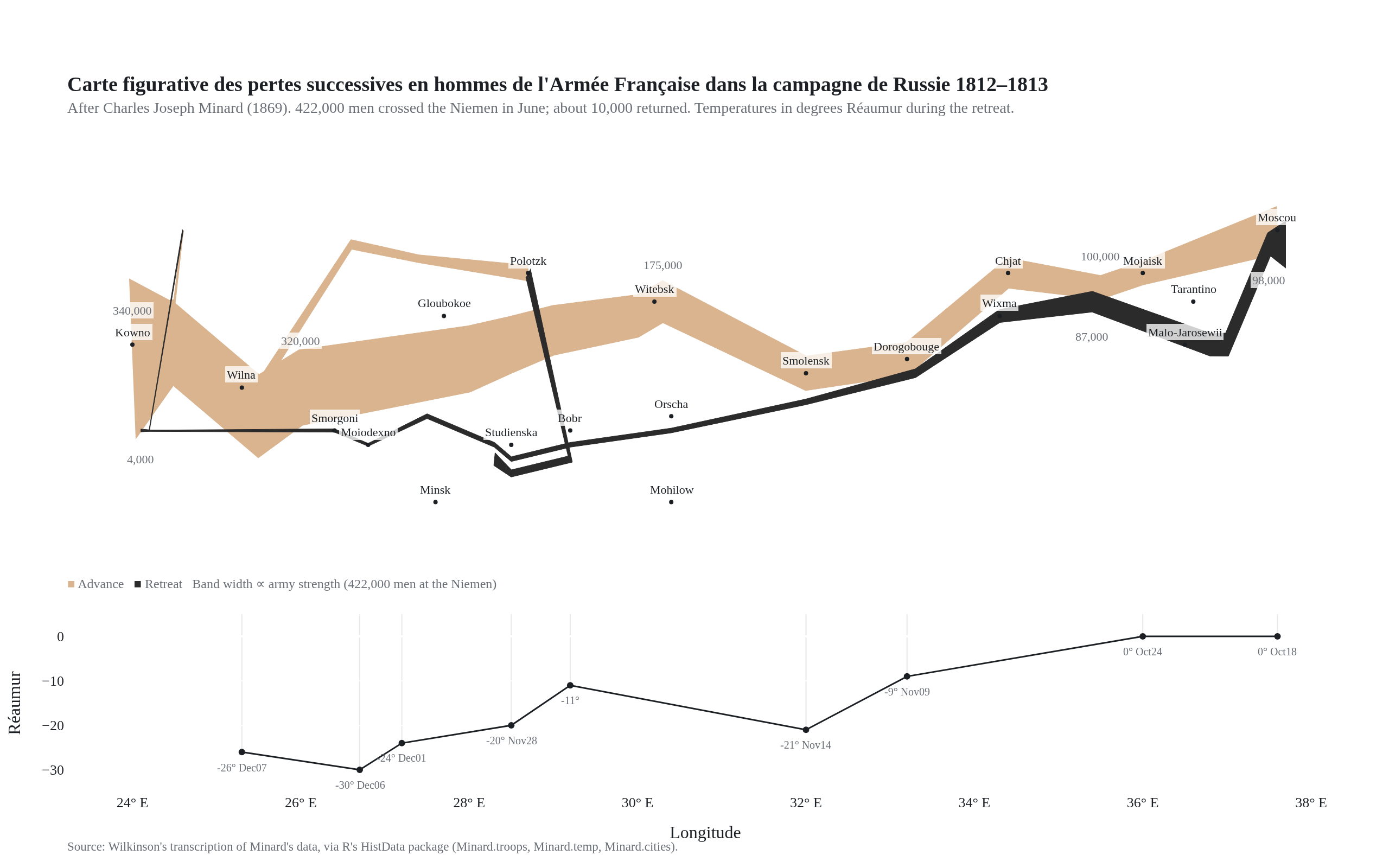
tapering bands as offset-curve polygons · advance and retreat as colour · city labels · a temperature panel aligned on longitude · serif type

Redrawing of Minard's map of Napoleon's 1812 Russian campaign: a tan band narrowing eastward to Moscow and a black band narrowing on the retreat, with a temperature chart beneath

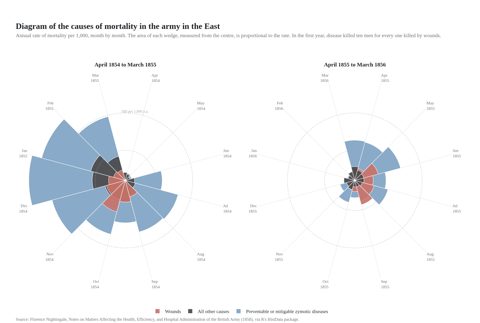
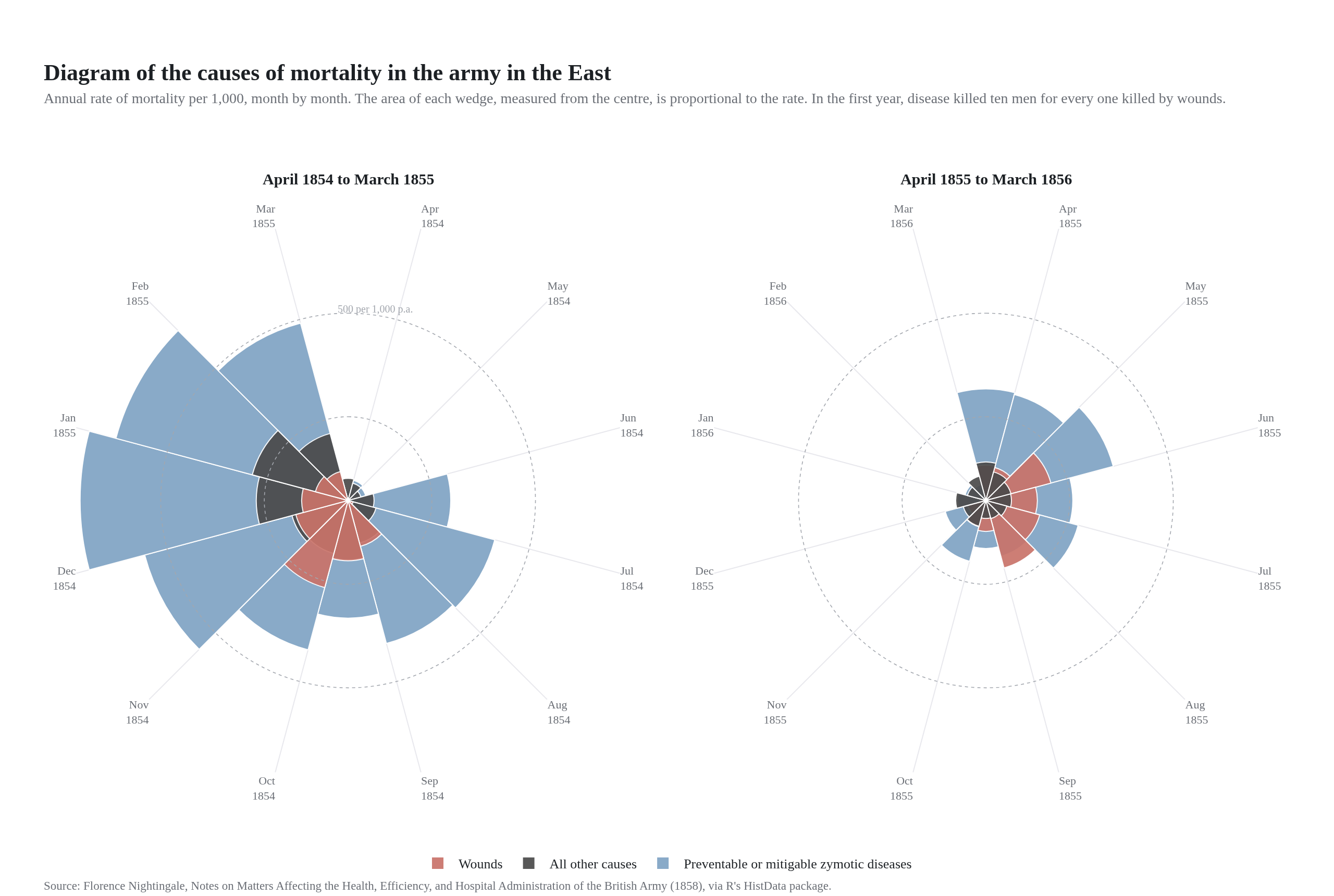
Nightingale's rose

HistData · Code · SVG · PNG

two polar subplots · wedges from the centre with area ∝ rate · Nightingale's three colours · dotted area guides · horizontal legend

Two rose diagrams after Florence Nightingale showing monthly army deaths from disease, wounds and other causes for April 1854 to March 1856

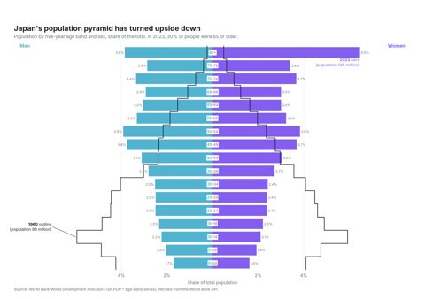
Population pyramid

World Bank API · Code · SVG · PNG
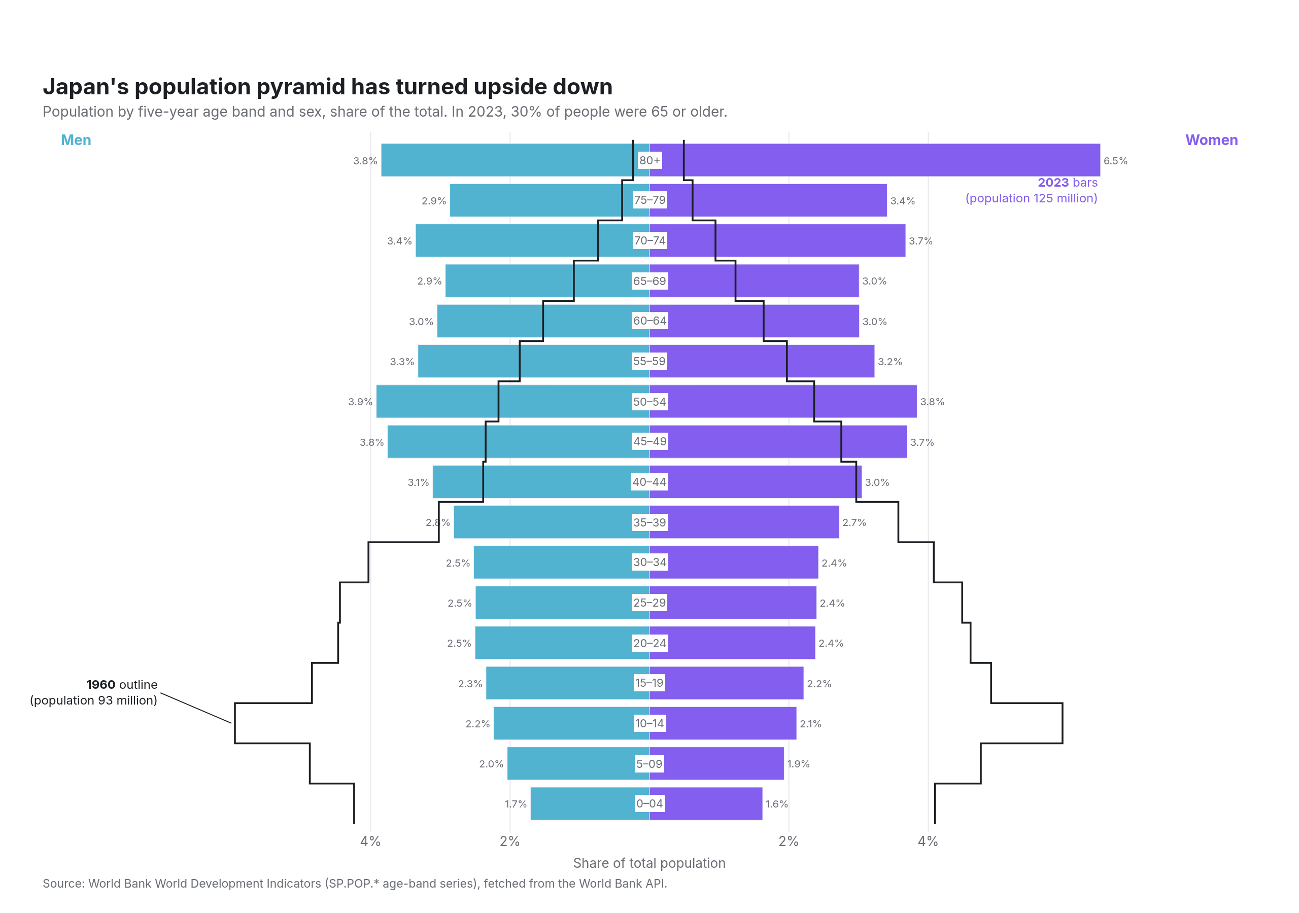
34 World Bank API calls · overlay bar mode · 1960 as a stepped outline · age bands labelled down the centre · mirrored percentage axis

Population pyramid of Japan with 2023 as filled bars for men and women and 1960 as a black stepped outline, showing the shift from a young to an old population

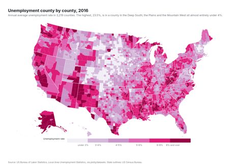
County choropleth

BLS via plotly/datasets · Code · SVG · PNG
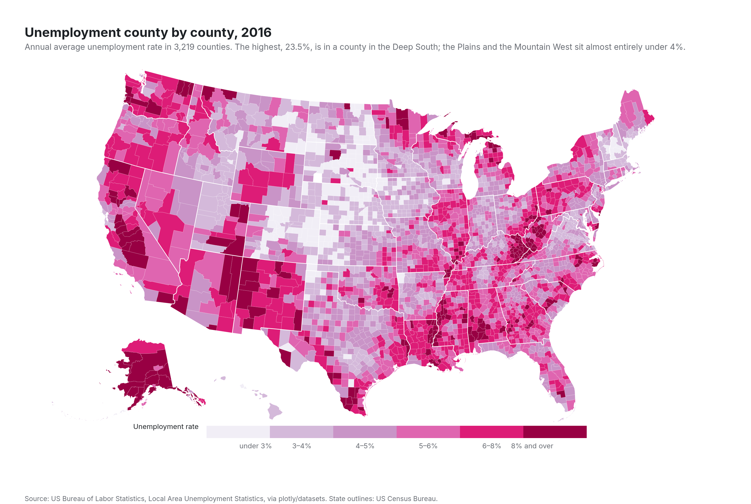
3,219 county polygons · Albers USA · six-class stepped colorscale · state borders as a line trace on top · swatch legend built from shapes

Choropleth map of the United States with every county coloured by its 2016 unemployment rate on a six-step purple-to-red scale, with a swatch legend along the bottom

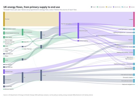
Energy Sankey

plotly.js sankey_energy mock (DECC) · Code · SVG · PNG
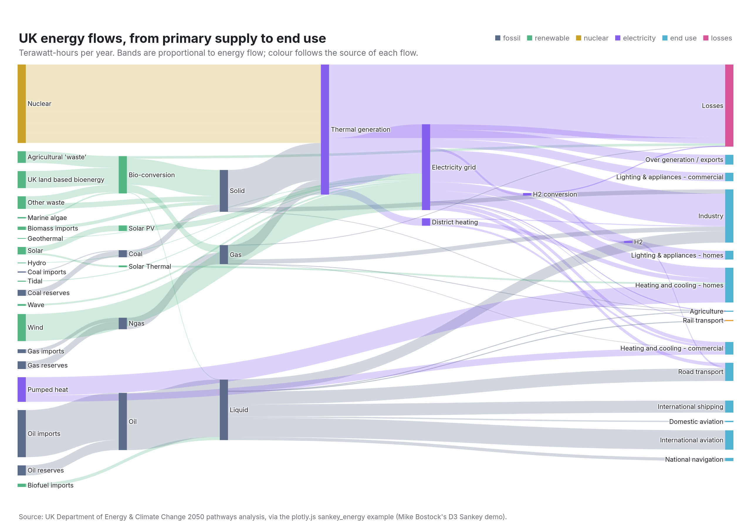
nodes coloured by kind · links inherit a translucent source colour · snap arrangement · inline colour key

Sankey diagram of UK energy flows from primary sources on the left through carriers to end uses and losses on the right

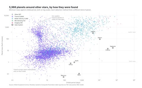
Exoplanet scatter

NASA Exoplanet Archive · Code · SVG · PNG
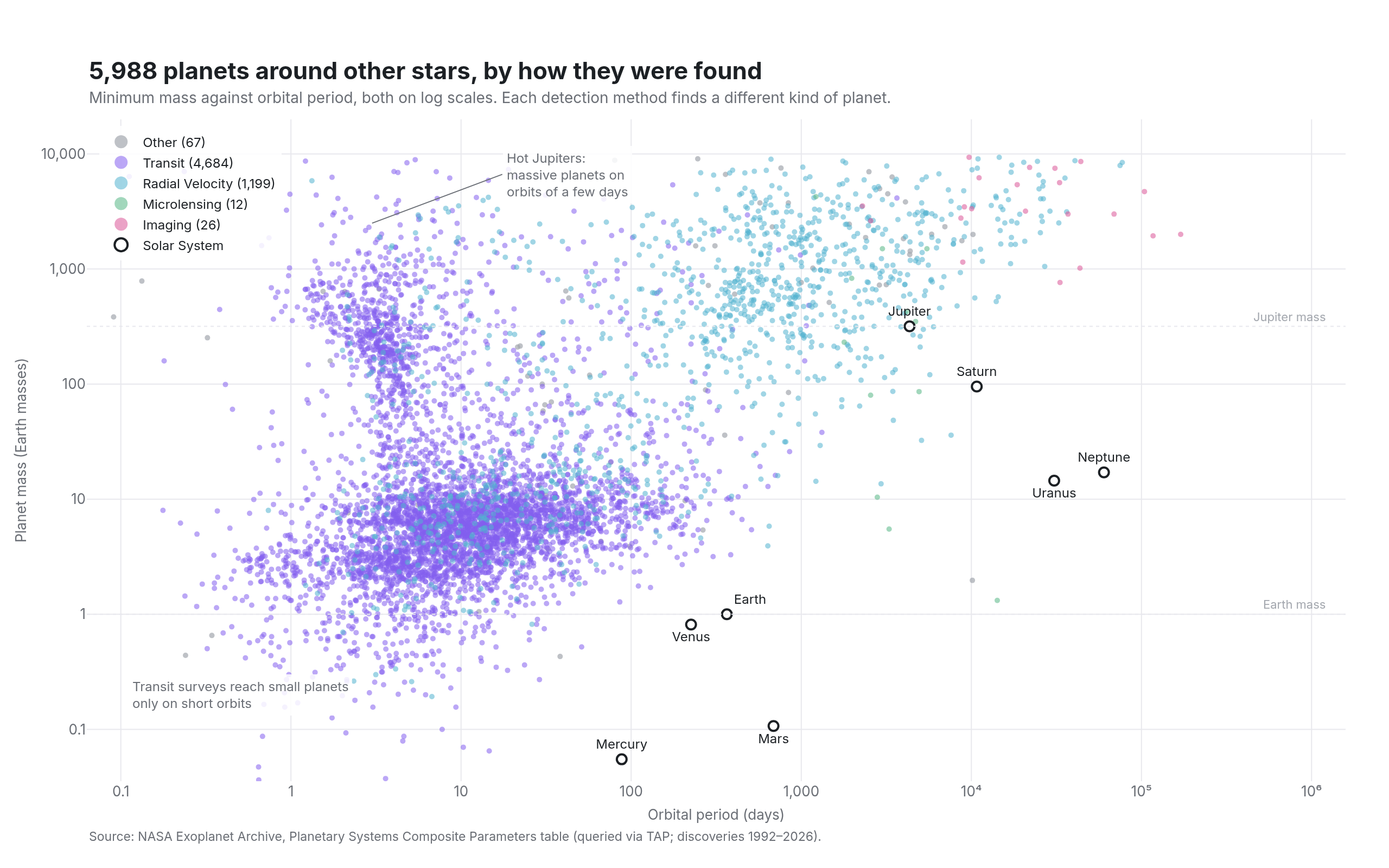
6,000 points on log–log axes · colour by detection method with counts in the legend · Solar System reference marks · dotted mass guides

Log-log scatter of planet mass against orbital period for about six thousand exoplanets coloured by discovery method, with the Solar System planets drawn as labelled rings

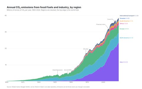
Stacked area with direct labels

Global Carbon Budget via Our World in Data · Code · SVG · PNG
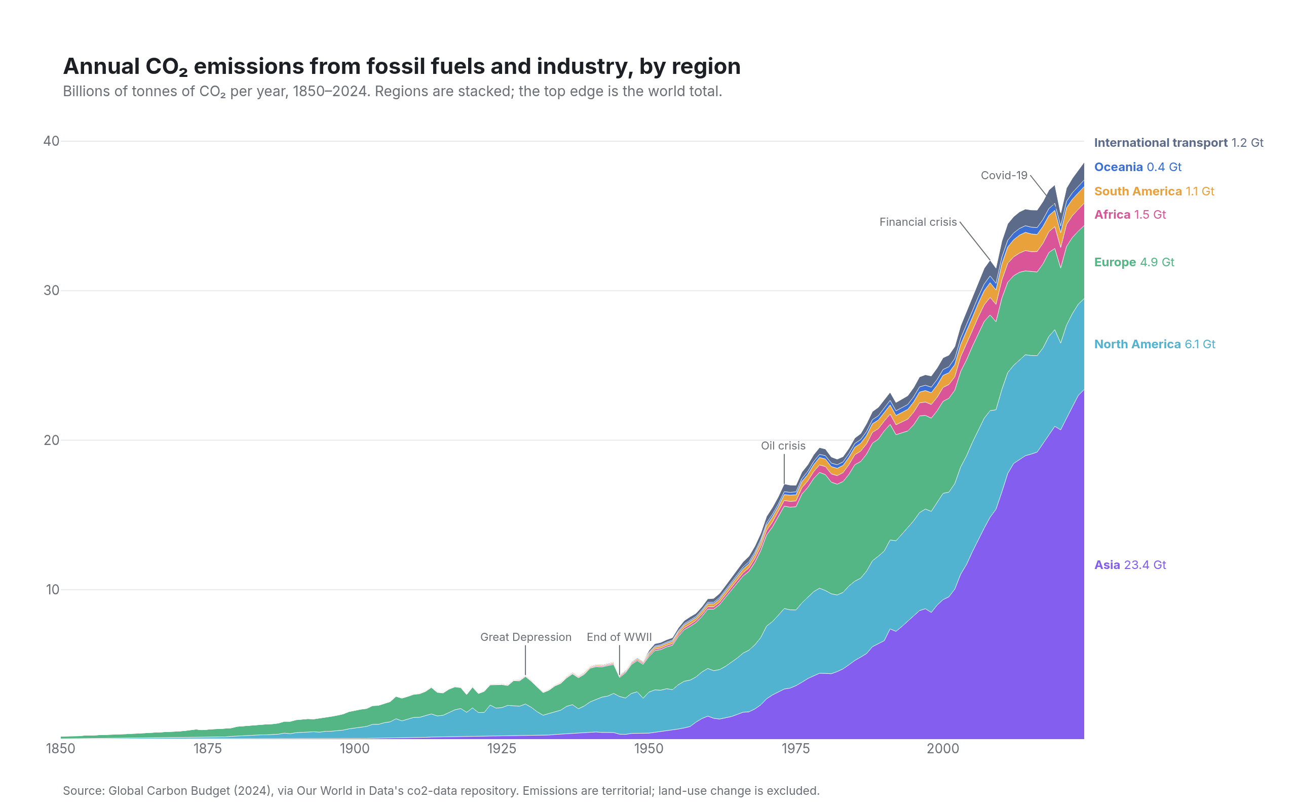
stackgroup areas · labels at the right edge, nudged apart · residual computed against the world total · dated events pinned to the top edge

Stacked area chart of annual CO₂ emissions from 1850 to 2024 by world region, Asia at the bottom in violet and each region labelled at the right edge

Journal figure

synthetic, seeded · Code · SVG · PNG
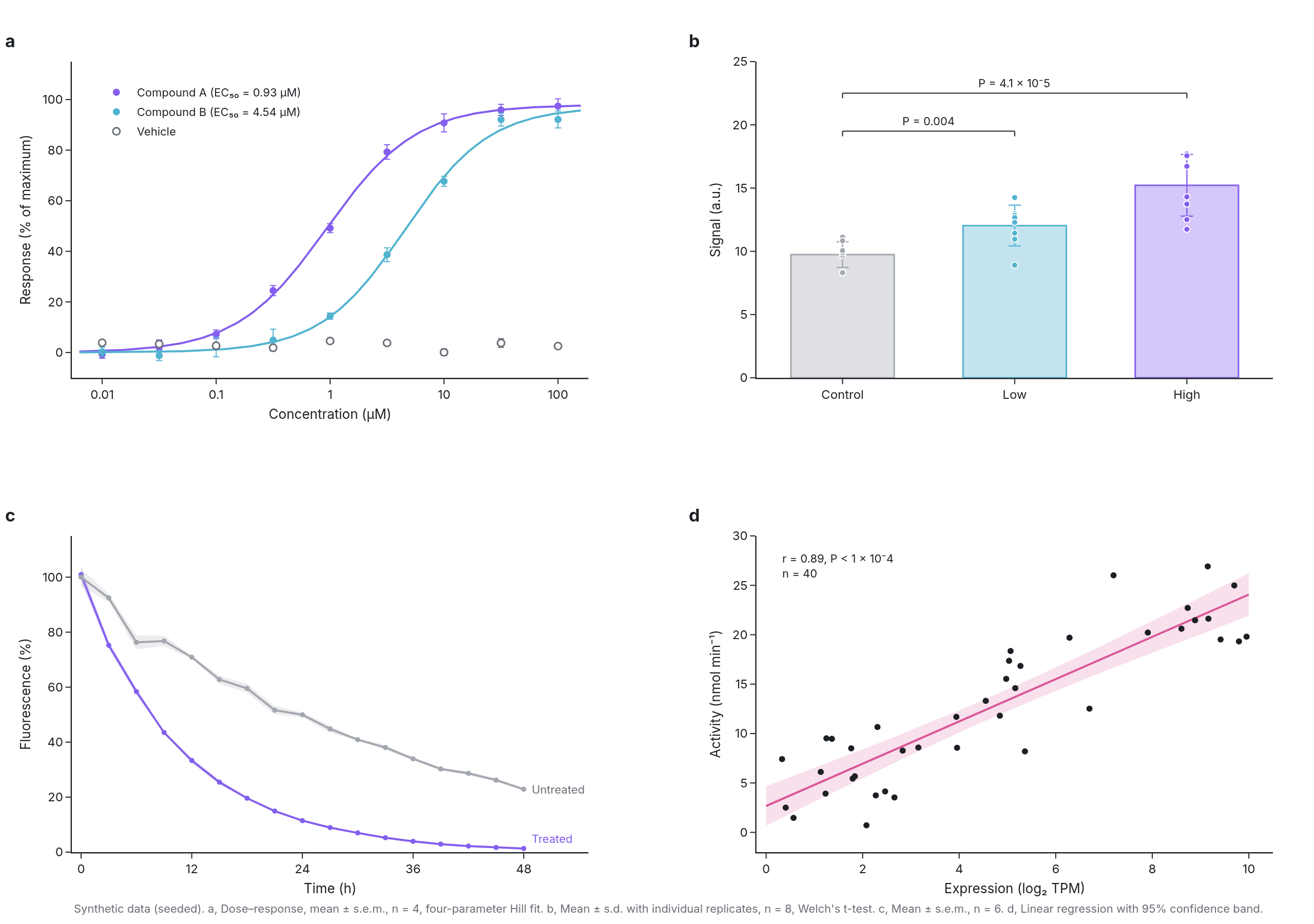
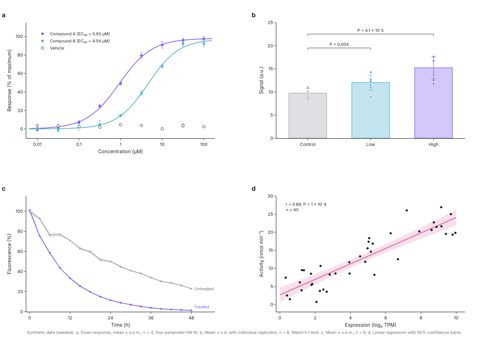
four lettered panels · Hill-curve fit · error bars · significance brackets from shapes · s.e.m. band · regression with 95% CI · figure legend

Four-panel scientific figure labelled a to d: a dose-response curve with a Hill fit, a bar chart with replicate points and p-value brackets, a time course with a shaded error band, and a regression with a confidence band

Raincloud plot

palmerpenguins via seaborn-data · Code · SVG · PNG
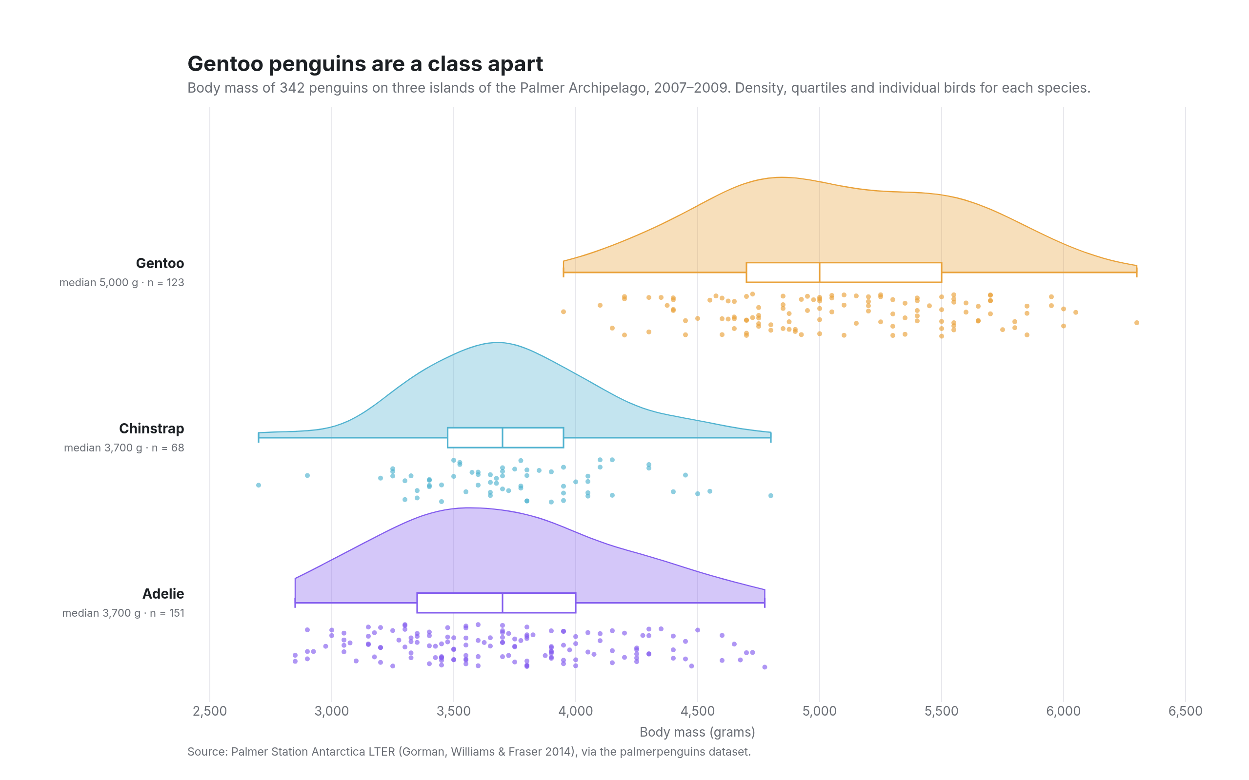
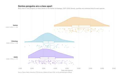
half violins · slim boxes · jittered points · numeric y positions under categorical labels · per-group medians

Raincloud plot of penguin body mass for Adelie, Chinstrap and Gentoo penguins, each with a half violin above a box plot and a cloud of individual points below

Ridgeline plot

nycflights13 weather table · Code · SVG · PNG
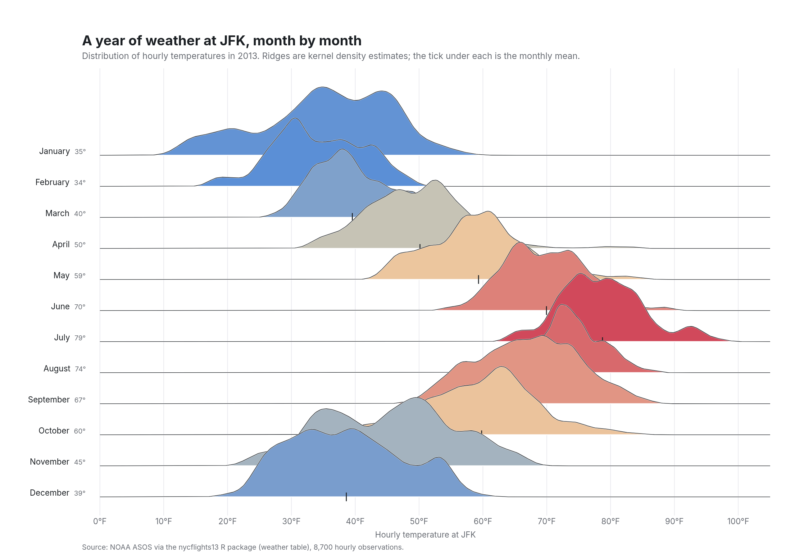
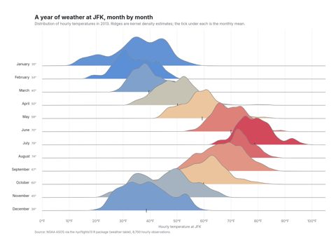
twelve KDE ridges as filled traces · overlap by drawing order · temperature-coloured ramp · month labels in place of an axis

Ridgeline plot of hourly temperatures at JFK airport in 2013, twelve overlapping density curves from January at the top to December at the bottom, coloured blue for cold months and red for hot

Bump chart

Our World in Data · Code · SVG · PNG
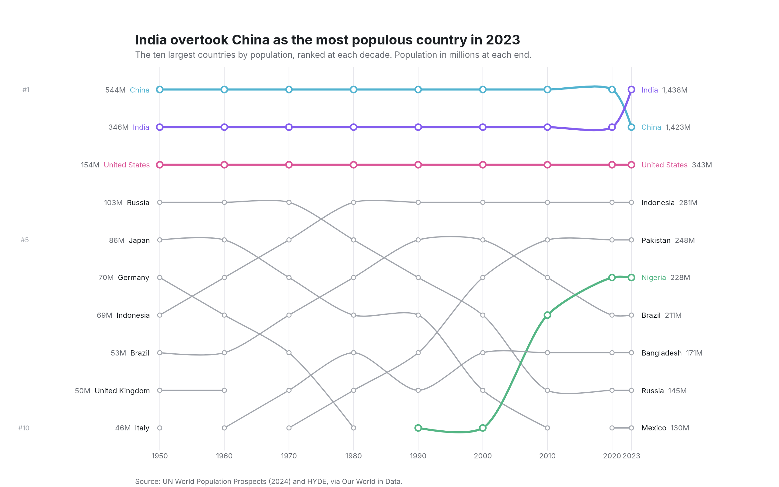
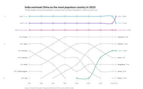
reversed rank axis · spline lines that break when a country drops out · labels with populations at both ends · four highlights

Bump chart ranking the ten most populous countries at each decade from 1950 to 2023, with India crossing above China at the end and Nigeria rising into the top ten

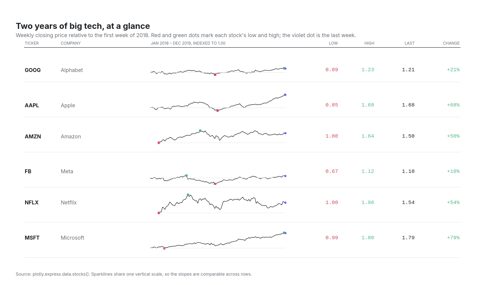
Sparkline table

plotly.express stocks · Code · SVG · PNG
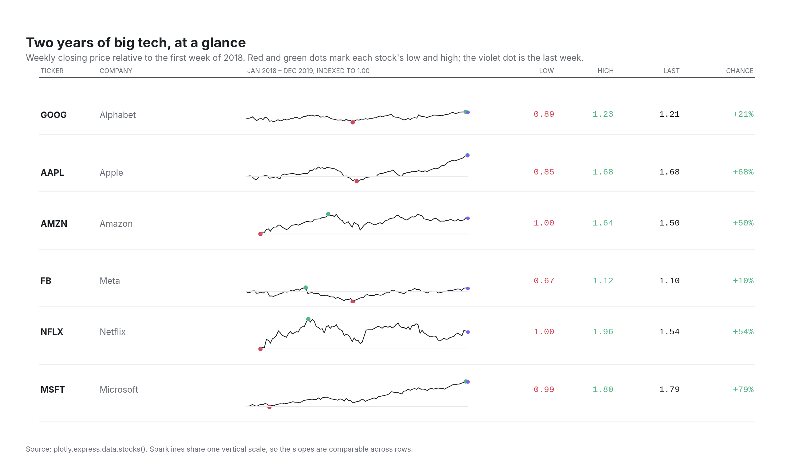
six subplot rows on one shared scale · text columns as annotations · low, high and last markers · tabular monospace figures · no axes at all

Table of six technology stocks with a small sparkline in each row, the low and high marked with red and green dots, and columns for the low, high, last price and percentage change

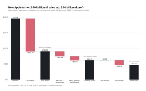
Waterfall chart

Apple Form 10-K, FY2024 · Code · SVG · PNG
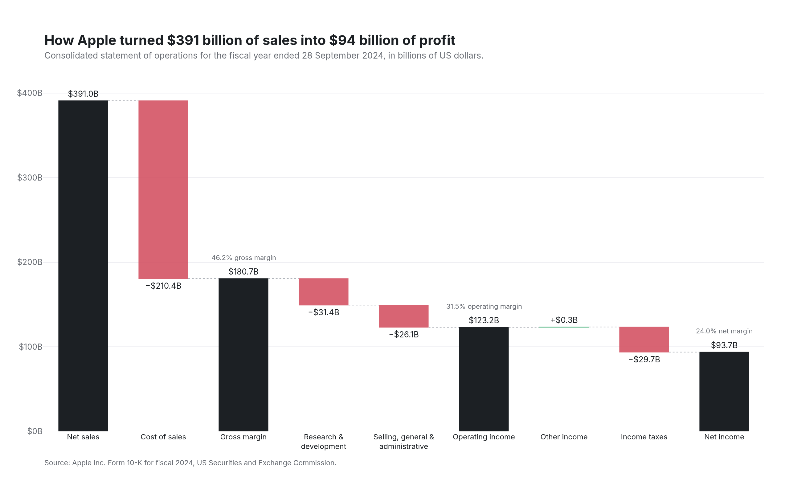
absolute, relative and total measures · dotted connectors · totals in ink, costs in red · margins written beside the totals

Waterfall chart of Apple's fiscal 2024 income statement from 391 billion dollars of net sales down through costs and taxes to 94 billion of net income

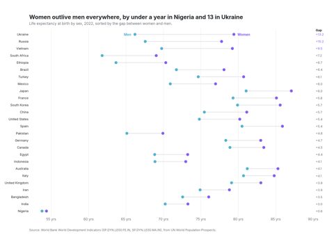
Dumbbell chart

World Bank API · Code · SVG · PNG
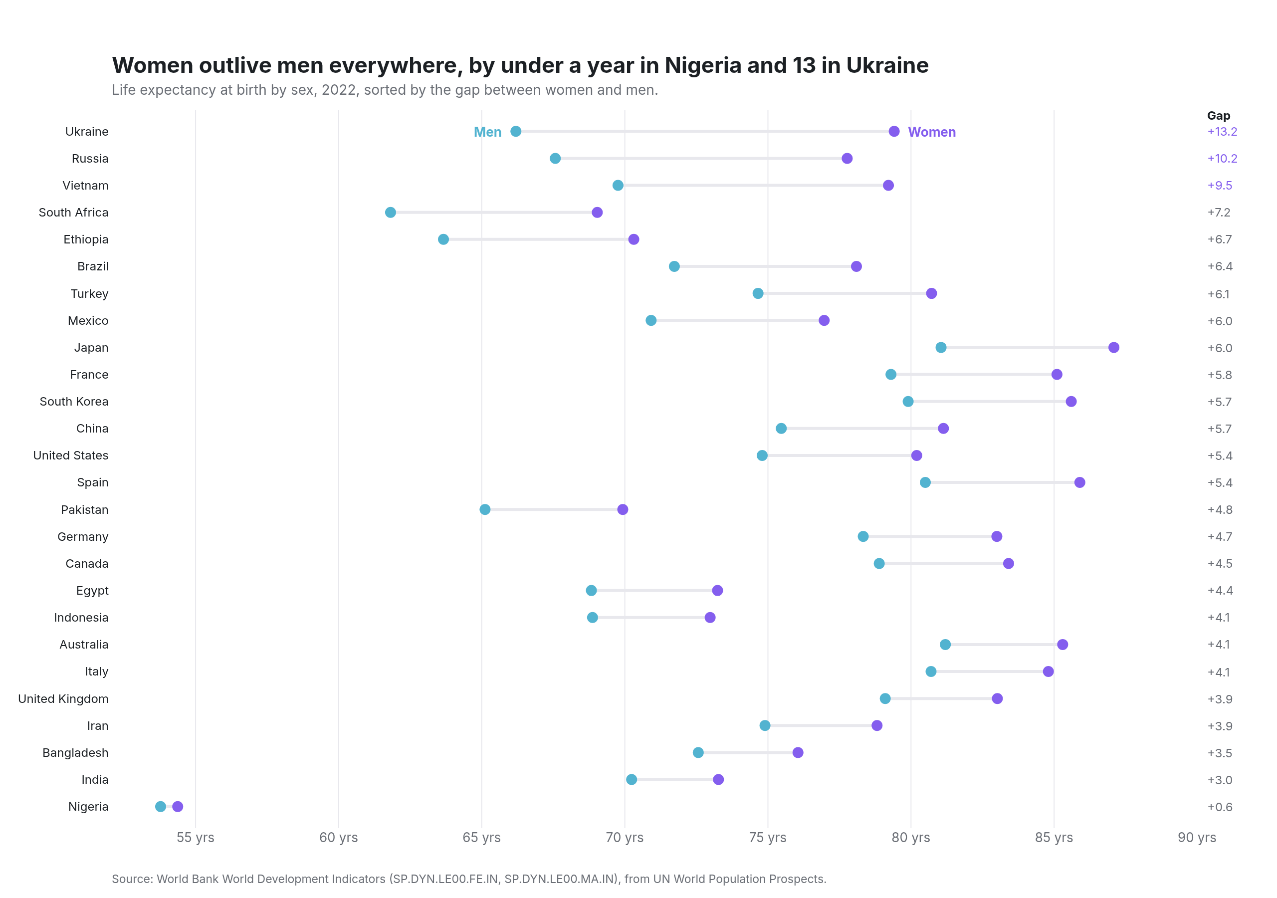
sorted by gap · one rule per row · sexes named once in the header · gap column at the right edge

Dumbbell chart of life expectancy for men and women in 26 countries in 2022, sorted by the size of the gap, with Ukraine at the top and Nigeria at the bottom

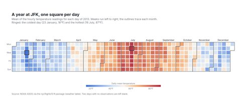
Calendar heatmap

nycflights13 weather table · Code · SVG · PNG
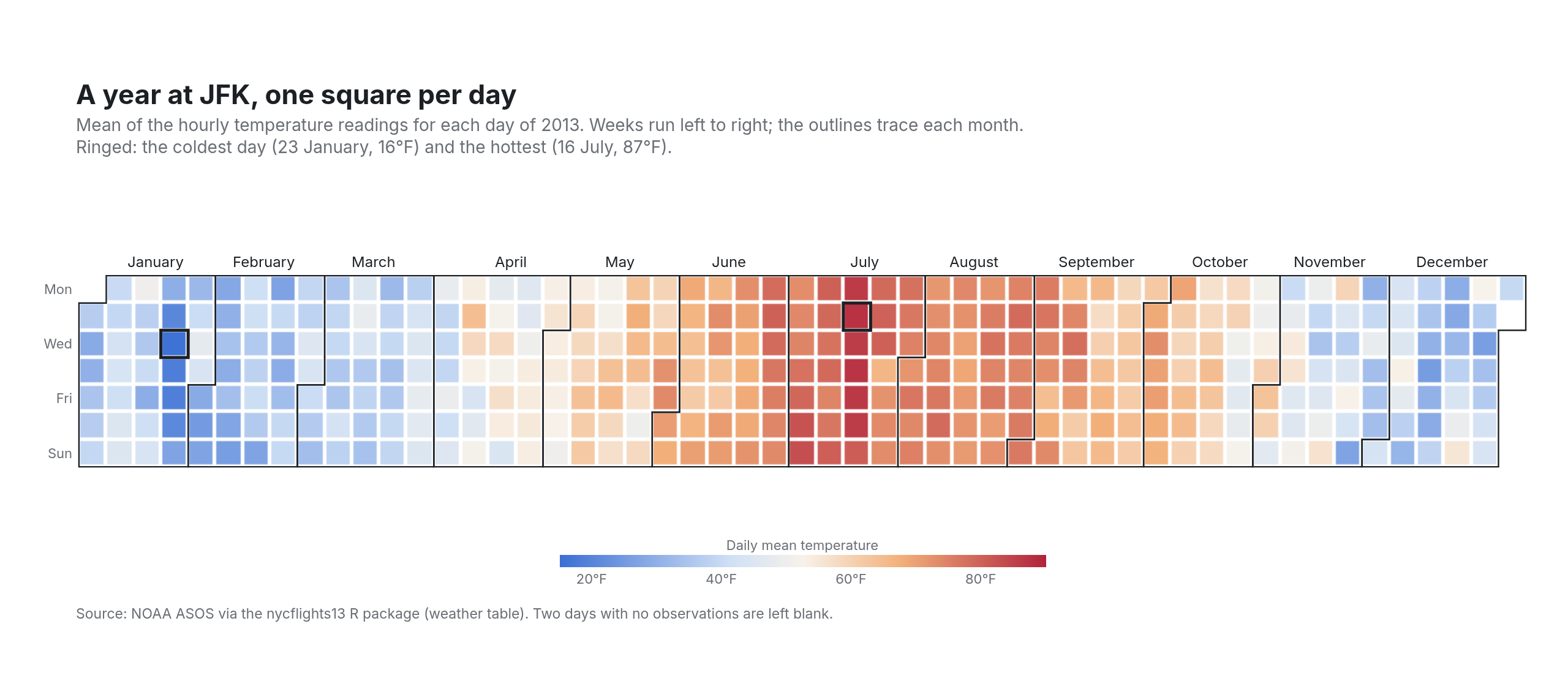
week × weekday heatmap · gaps as the grid · month outlines as SVG paths · month labels · extremes ringed with shapes · horizontal colour bar

Calendar heatmap of daily mean temperature at JFK airport in 2013 laid out like a GitHub contributions graph, with each month outlined in black

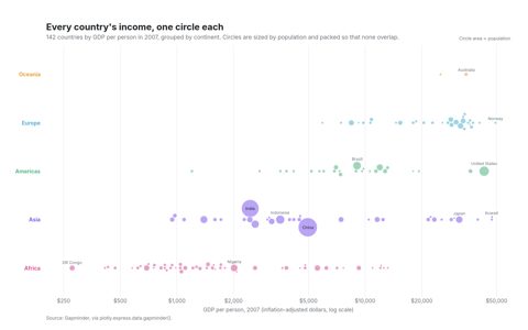
Beeswarm

Gapminder via plotly.express · Code · SVG · PNG
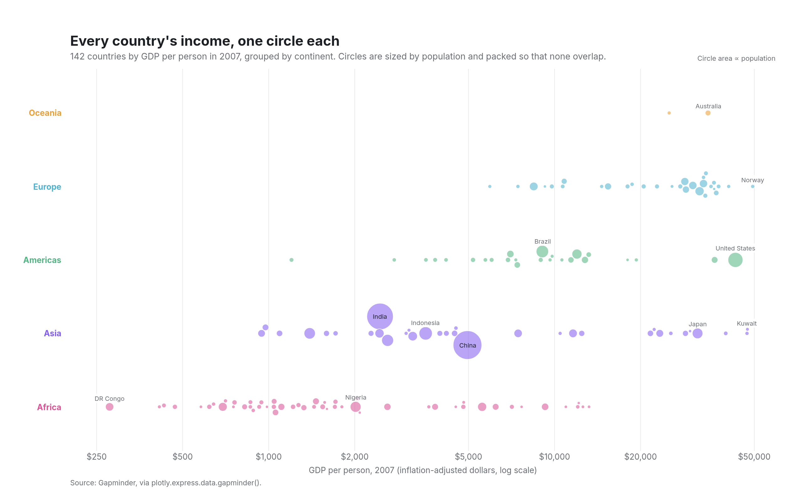
greedy circle packing in pixel space · log x axis · circle area ∝ population · continent rows · a few labelled circles

Beeswarm plot of GDP per person in 2007 for 142 countries in five continent rows on a log scale, with circles sized by population and China and India drawn largest

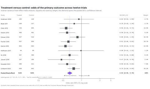
Forest plot

synthetic, seeded · Code · SVG · PNG
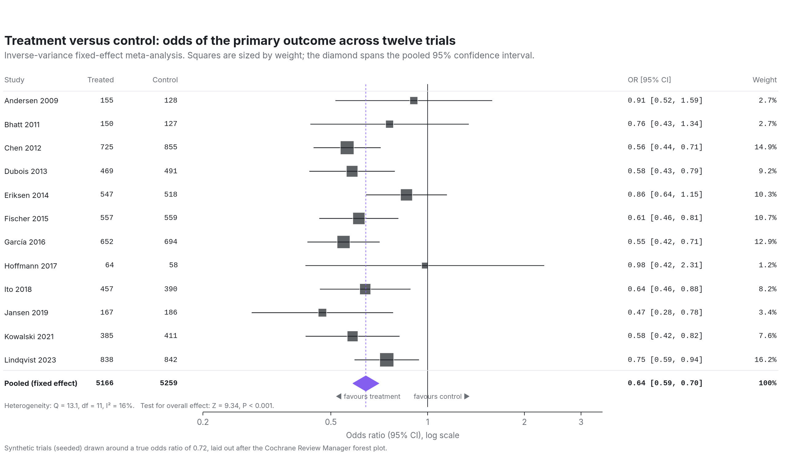
table columns in paper coordinates on both sides · squares sized by weight · pooled diamond as a polygon · log axis through 1 · heterogeneity line

Forest plot of twelve trials with each study's odds ratio and confidence interval, squares sized by weight, and a violet diamond for the pooled estimate below

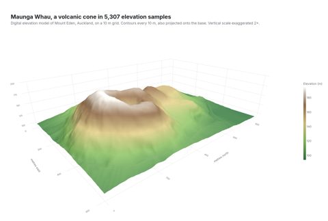
Terrain surface

R datasets::volcano · Code · SVG · PNG
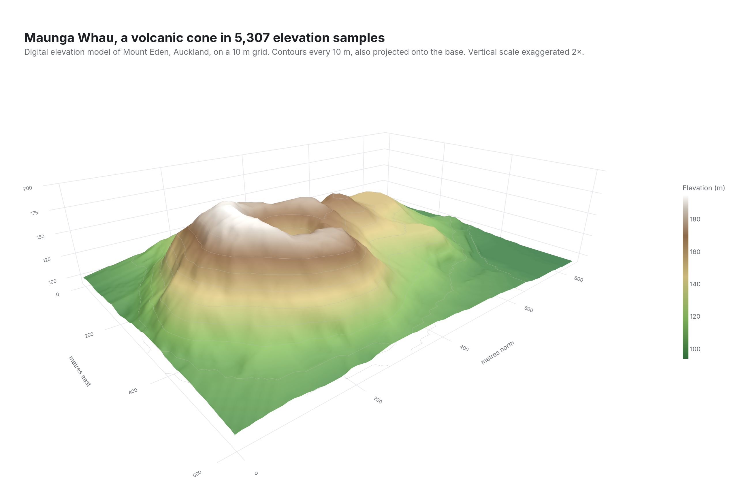
3D surface · terrain colour ramp · Phong lighting from the north-west · contours on the surface and projected to the floor · vertical exaggeration · low camera

Three-dimensional relief model of Maunga Whau, a volcanic cone in Auckland, coloured from green lowlands through brown slopes to a white rim, with contour lines and a crater visible from a low viewpoint

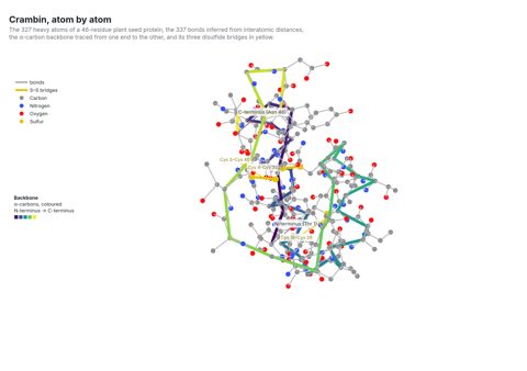
Ball and stick molecule

RCSB Protein Data Bank, 1CRN · Code · SVG · PNG
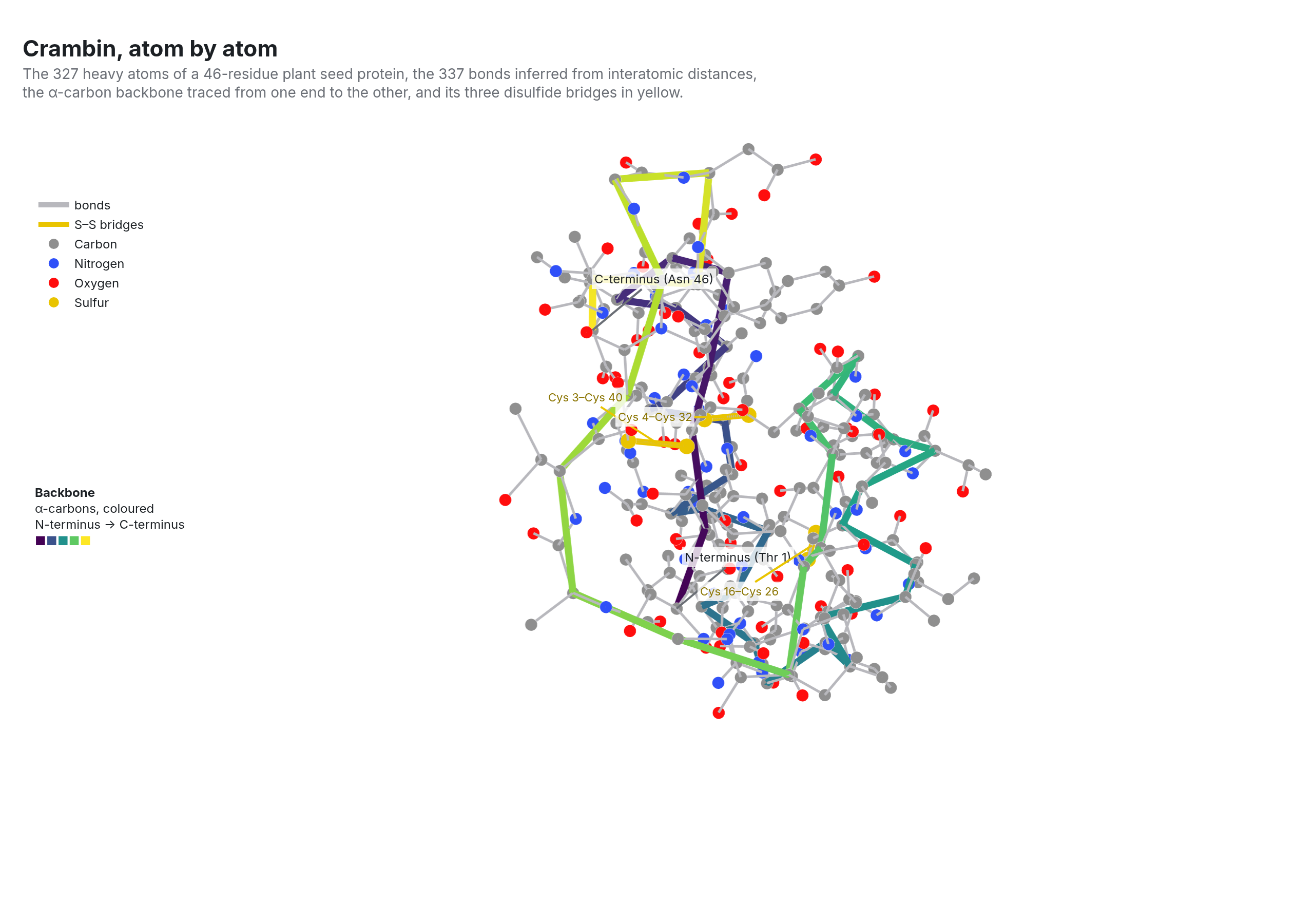
atoms parsed from a PDB file · bonds inferred by distance as one None-gapped scatter3d · CPK colours · backbone tube coloured along the chain · 3D annotations · no axes

Ball-and-stick model of the protein crambin: grey, blue, red and yellow spheres for carbon, nitrogen, oxygen and sulfur atoms joined by grey bonds, with the backbone drawn as a thick tube coloured from purple to yellow and three disulfide bridges labelled

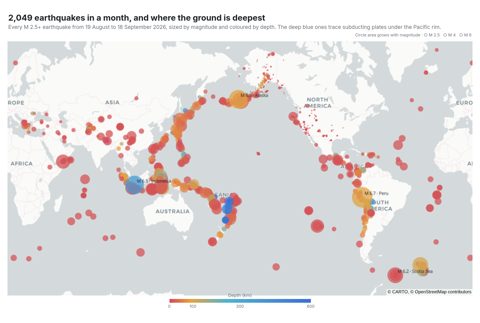
Earthquake map

USGS real-time feed, M2.5+ past month · Code · SVG · PNG
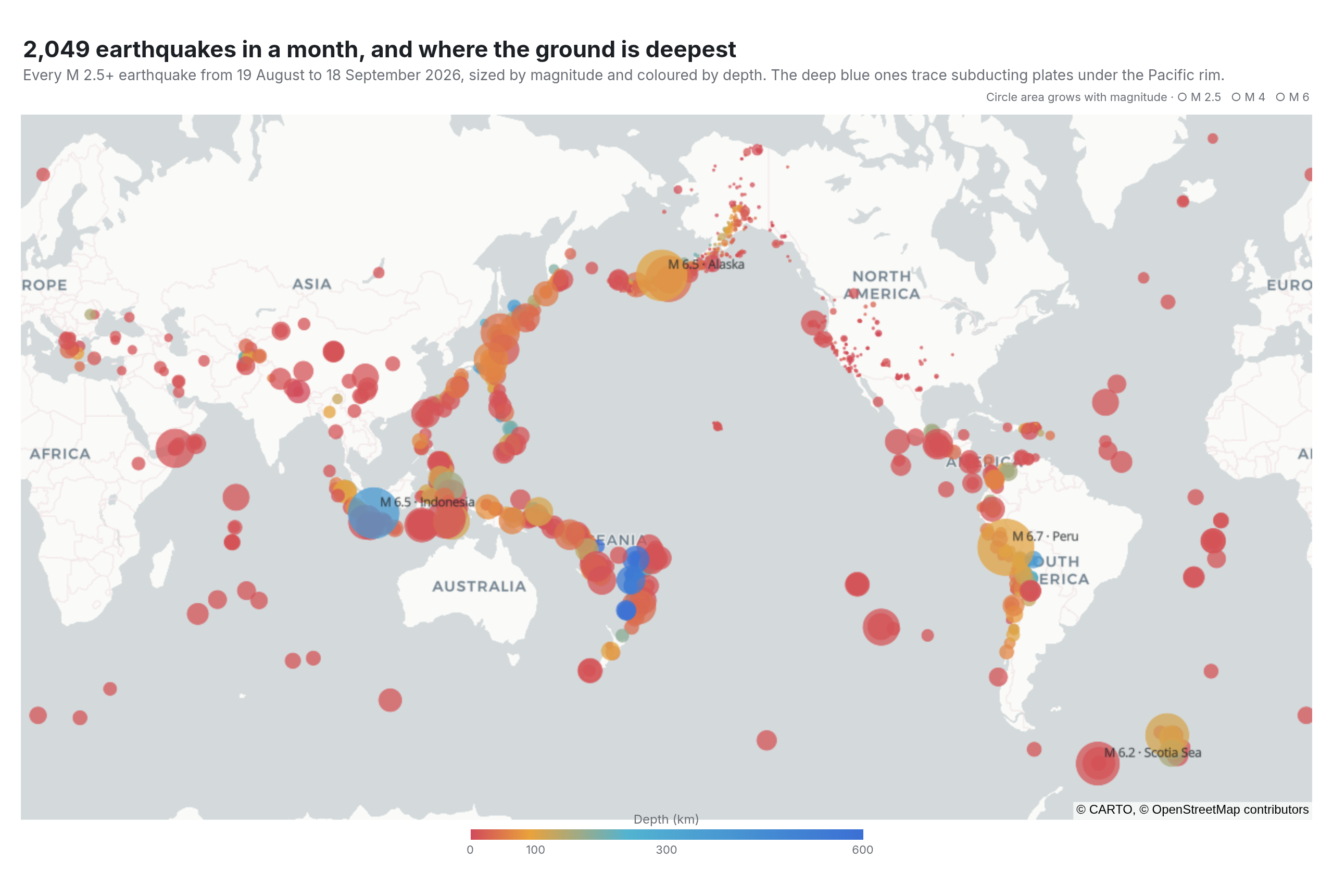
MapLibre `map` trace, no token · Carto basemap · circles sized by magnitude and coloured by depth · a second text-only layer for the largest events · Pacific-centred view · horizontal colour bar

World map centred on the Pacific Ocean with a month of earthquakes drawn as circles sized by magnitude and coloured from red for shallow to blue for deep, the largest labelled with their magnitude and region

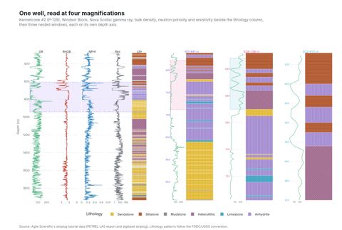
Borehole striplog

Kennetcook #2 (P-129), Agile striplog · also in the compendium · Code · SVG · PNG
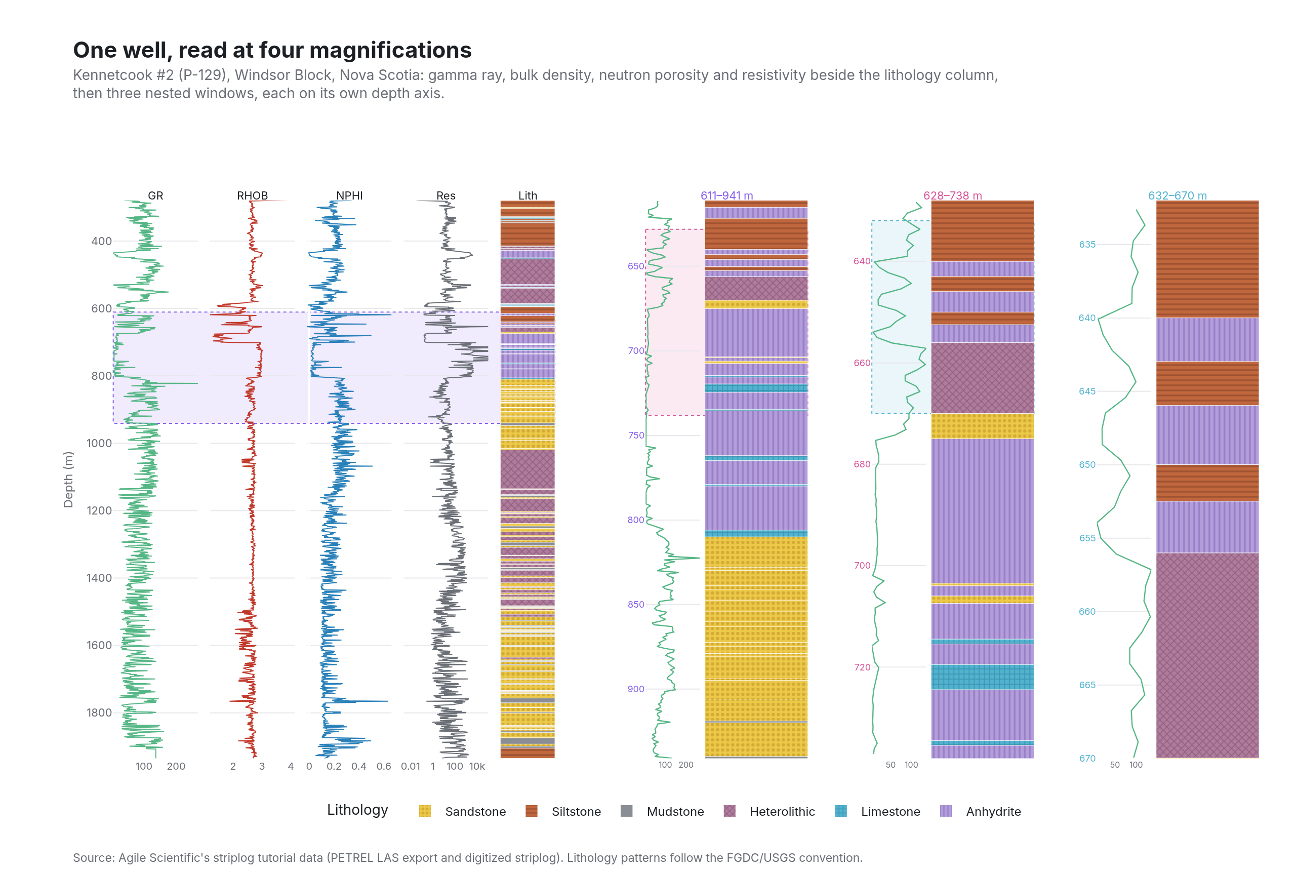
eleven x axes and four y axes, every domain placed by hand · reversed shared depth axis · USGS lithology patterns · nested zoom windows · highlight bands as shapes

Composite well log for the Kennetcook #2 borehole: four wireline curves beside a patterned lithology column on a reversed depth axis, with three highlighted intervals each expanded into its own zoomed panel to the right

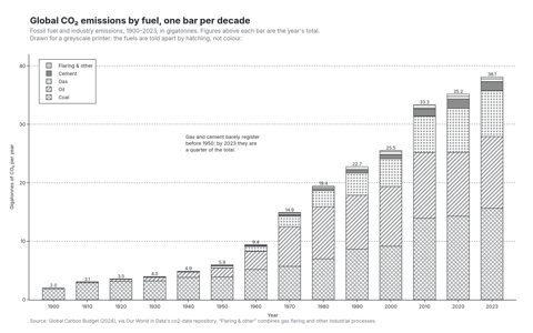
Pattern fills, black and white

Global Carbon Budget via Our World in Data · Code · SVG · PNG
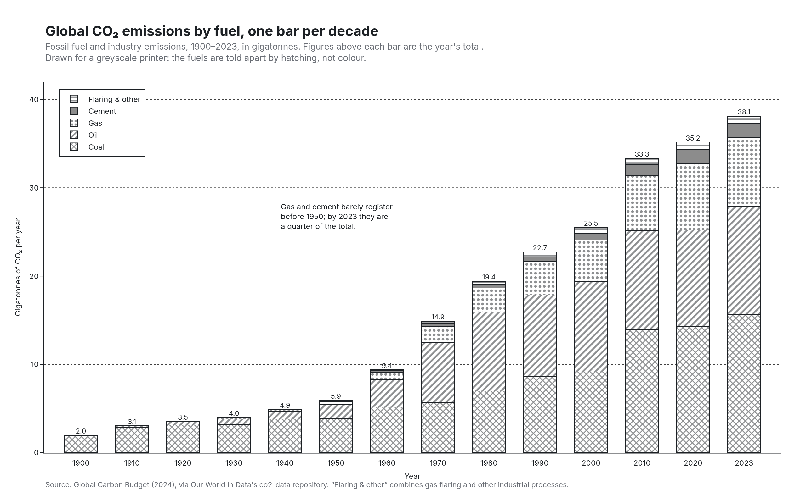
marker.pattern hatching instead of colour · stacked bars with ink outlines · dotted grid · boxed legend showing the same hatches · totals as a text trace

Black-and-white stacked bar chart of world CO₂ emissions by fuel for each decade from 1900 to 2023, with coal, oil, gas, cement and flaring distinguished by crosshatch, diagonal, dotted, grey and horizontal-line fills

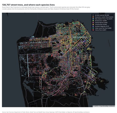
City map, 139,000 points

DataSF street tree census · Code · SVG · PNG
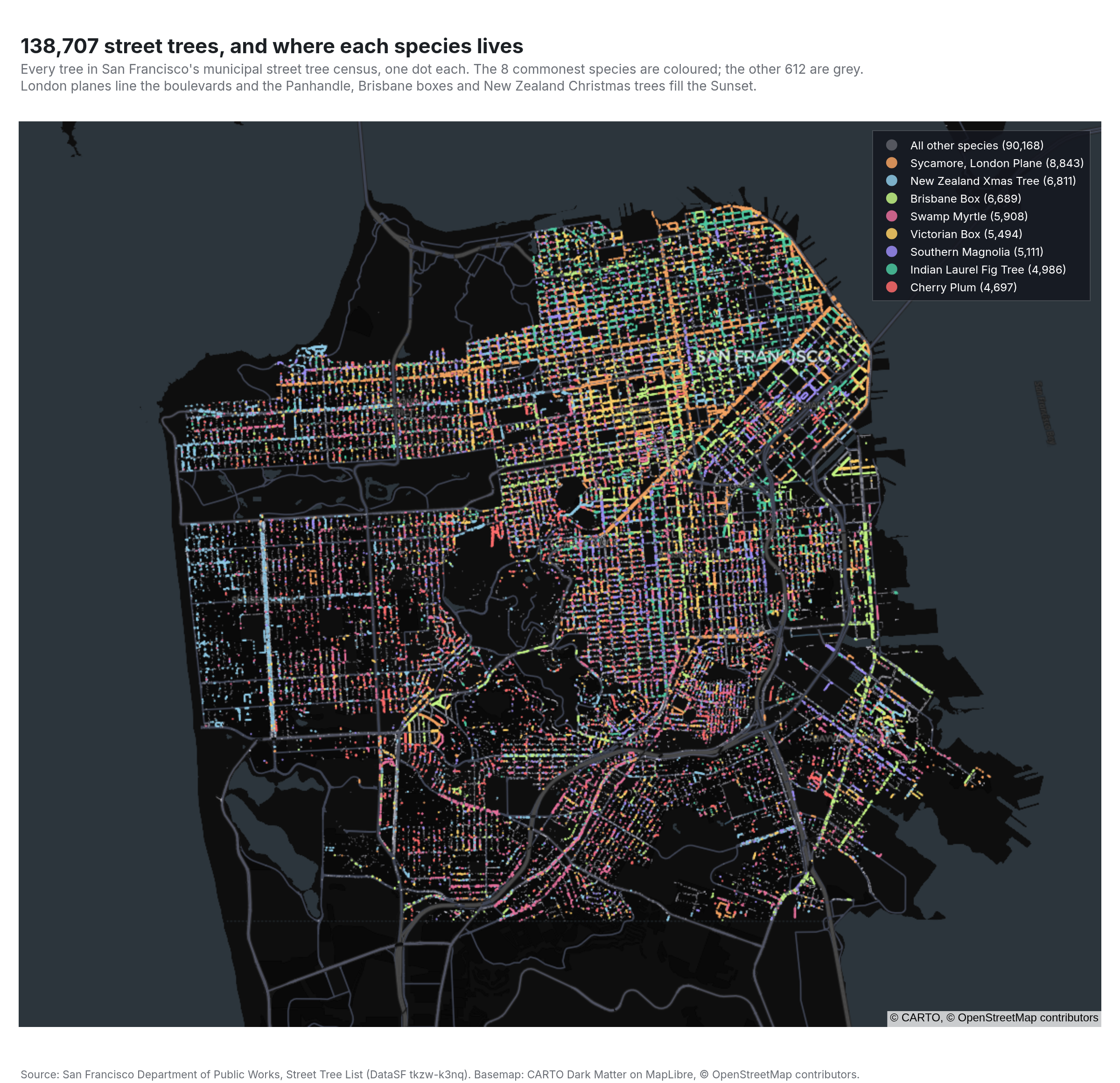
MapLibre `map` trace at city scale · nine scattermap layers, one per species · dark basemap with its own labels · legend with counts · the streets drawn by the data

Dark map of San Francisco with every street tree drawn as a small coloured dot, the eight commonest species in orange, blue, green, pink, yellow, purple, teal and red and the rest in grey, so the street grid appears from the trees alone

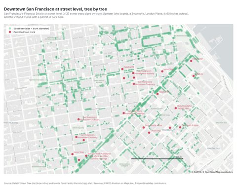
Street-level map

DataSF street trees · DataSF mobile food permits · Code · SVG · PNG
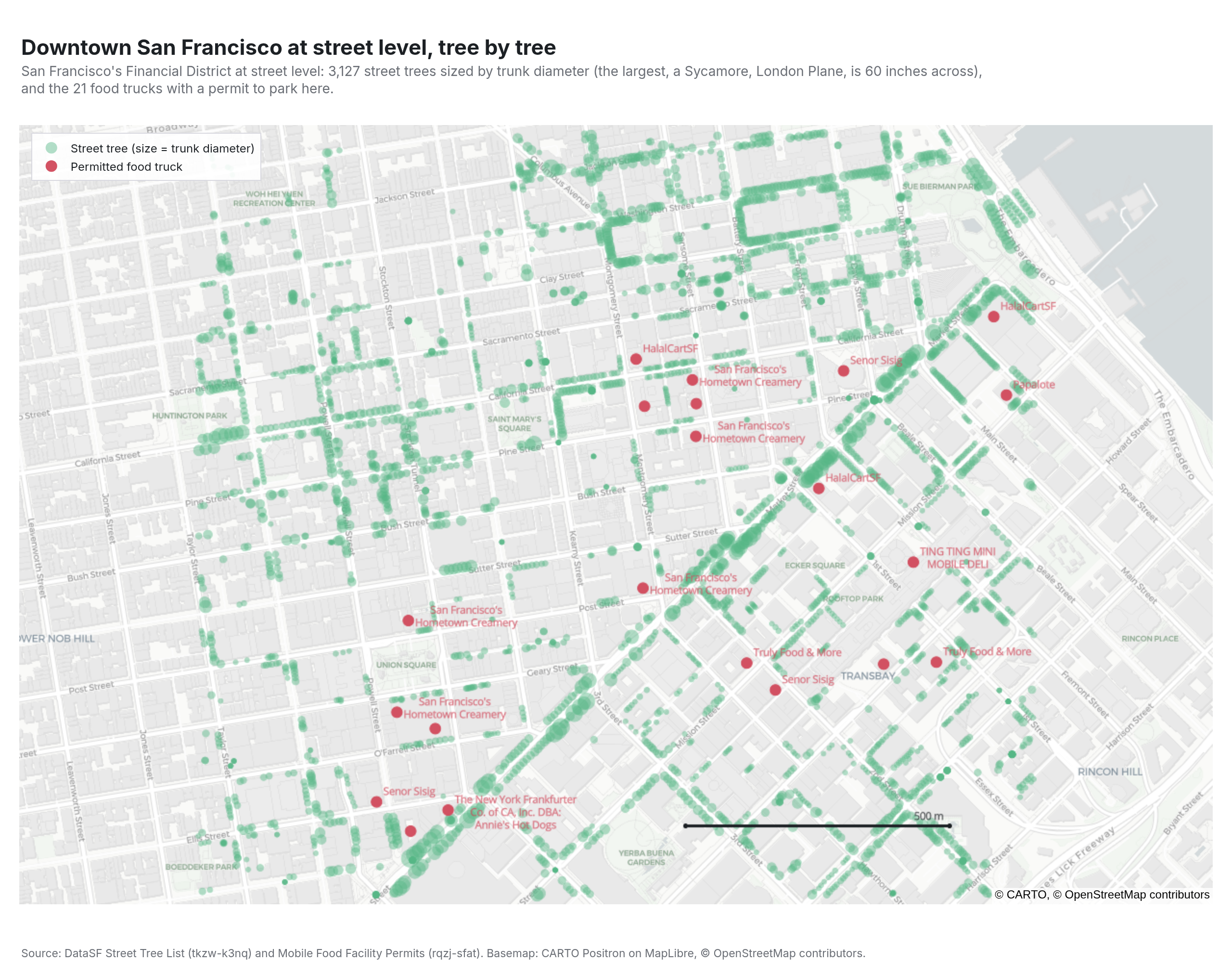
MapLibre `map` trace at zoom 15 · light basemap whose own street names do the wayfinding · markers sized by trunk diameter · labelled point layer · a scale bar computed from two coordinates

Street-level map of San Francisco's Financial District with every street tree drawn as a green circle sized by trunk diameter and the permitted food trucks as labelled red dots, over a light basemap showing street names

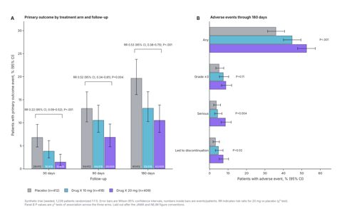
Clinical trial bar chart

synthetic, seeded · Code · SVG · PNG
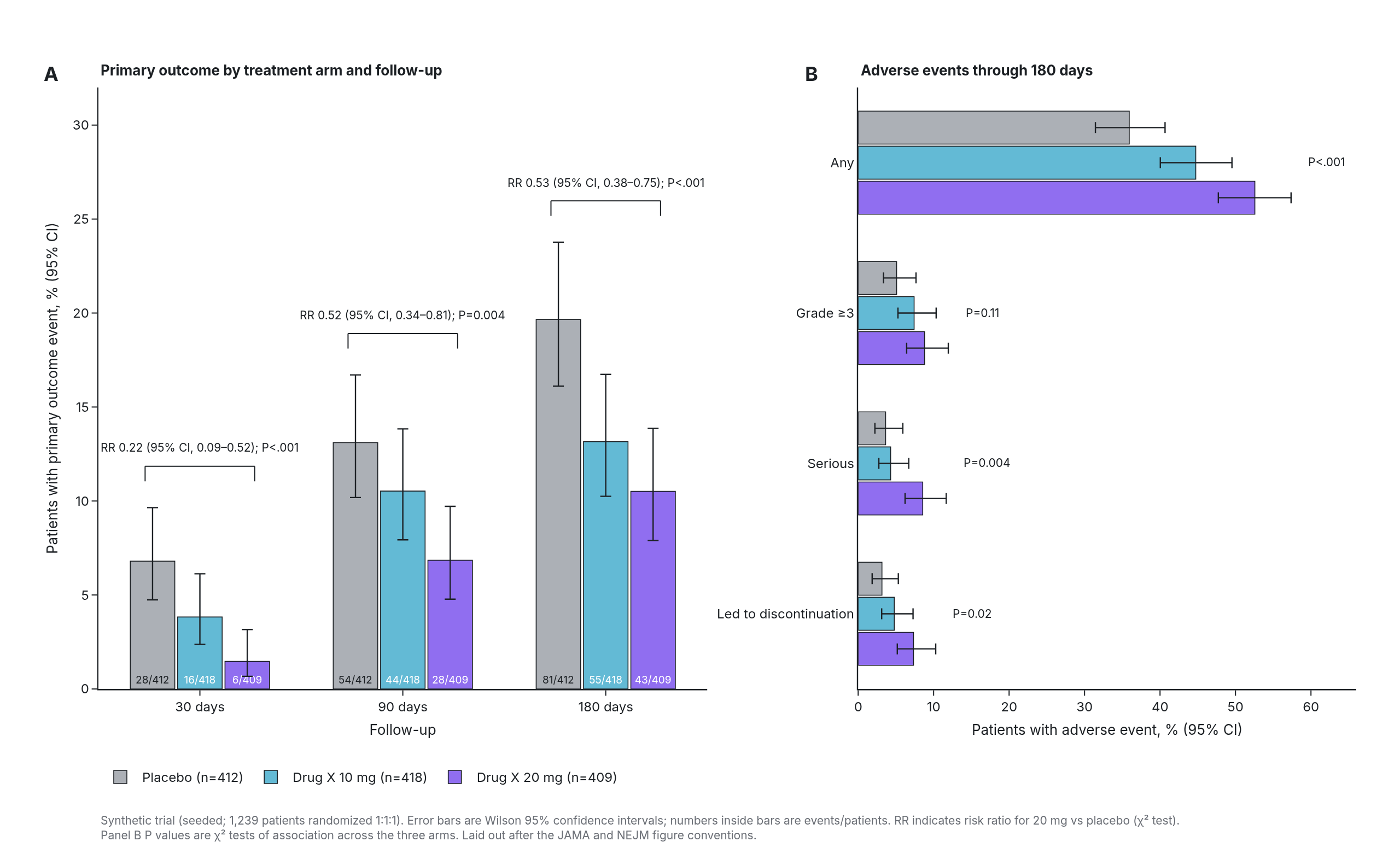
grouped bars with asymmetric Wilson 95% CIs · comparison brackets from shapes with risk ratios and exact P values · events/patients inside the bars · group sizes in the legend · lettered panels · horizontal bars for adverse events

Two-panel medical journal figure: panel A groups bars of primary outcome rates by treatment arm at 30, 90 and 180 days with confidence intervals and bracketed risk ratios; panel B shows horizontal bars of adverse event rates by grade for the three arms