
Journal figure
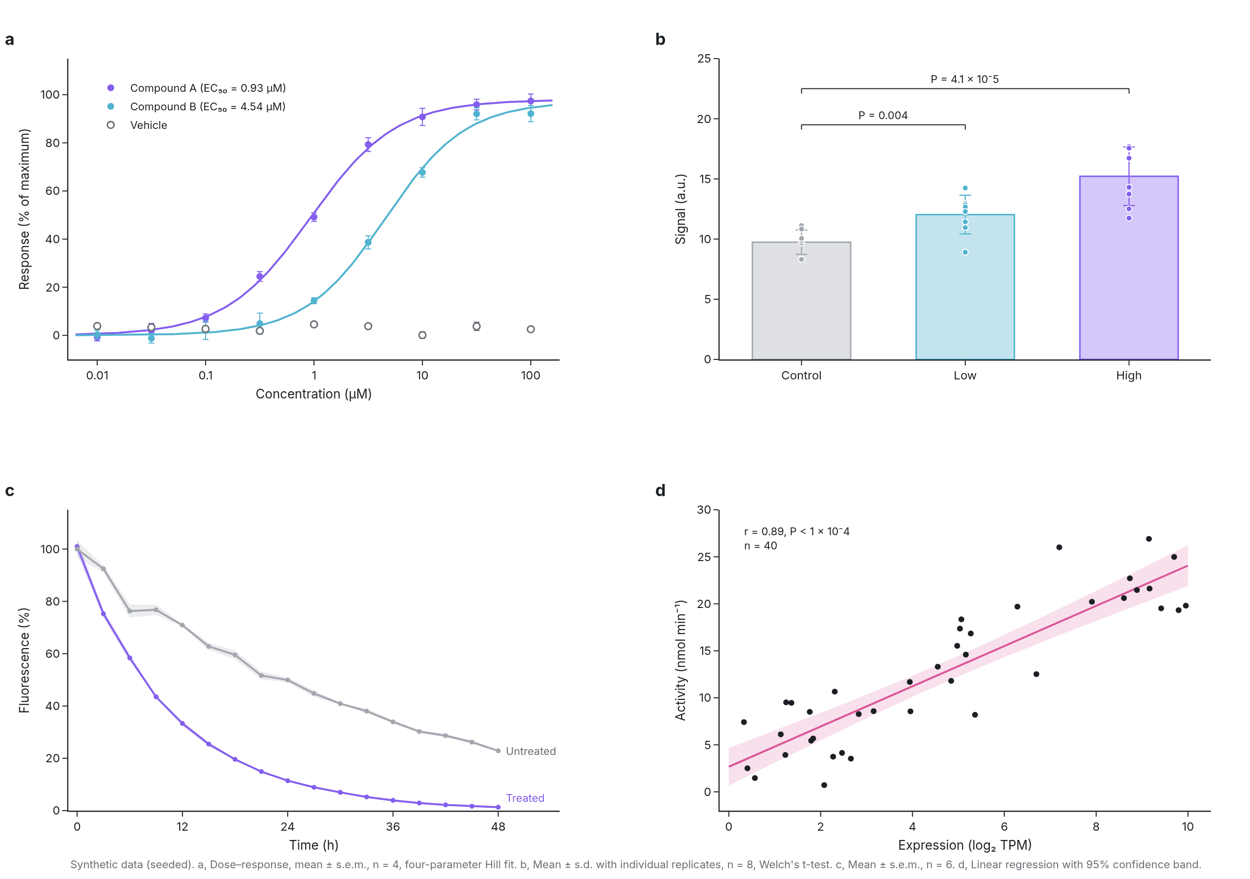
a four-panel Nature-style layout from one synthetic assay
Example from Plotly for highly customizable print-ready data visualization · shared helpers
Python Code
"""Journal figure — a four-panel Nature-style layout from one synthetic assay.

The conventions of a life-sciences figure: lettered panels, axis lines only
on the left and bottom, ticks pointing out, no gridlines, a fitted Hill curve
through mean ± s.e.m., significance brackets with p values, individual data
points over their summary bars, and a regression with its 95% confidence band.
"""
from pathlib import Path

from _shared import save, base_layout, panel_label, INK, MUTED, FAINT, VIOLET, TEAL, PINK, hex_to_rgba

import numpy as np
import plotly.graph_objects as go
from plotly.subplots import make_subplots
from scipy import stats
from scipy.optimize import curve_fit

CHART_NUM = 15
rng = np.random.default_rng(7)
COMPOUNDS = [("Compound A", VIOLET, 0.8), ("Compound B", TEAL, 5.0), ("Vehicle", FAINT, None)]
AX = dict(showgrid=False, showline=True, linecolor=INK, linewidth=1.2, ticks="outside", tickcolor=INK, ticklen=5,
          tickfont=dict(size=12, color=INK), title=dict(font=dict(size=13, color=INK), standoff=8), zeroline=False)


def hill(x, top, ec50, n):
    return top * x ** n / (ec50 ** n + x ** n)


def generate():
    fig = make_subplots(rows=2, cols=2, horizontal_spacing=0.14, vertical_spacing=0.2)

    # a) dose–response with Hill fit
    doses = np.logspace(-2, 2, 9)
    for name, color, ec50 in COMPOUNDS:
        if ec50 is None:
            y = rng.normal(3, 2.5, size=(9, 4)); mean, sem = y.mean(1), y.std(1, ddof=1) / 2
            fig.add_trace(go.Scatter(x=doses, y=mean, mode="markers", name=name, marker=dict(size=7, color="white", line=dict(color=MUTED, width=1.5)),
                                     error_y=dict(type="data", array=sem, color=MUTED, thickness=1, width=3)), row=1, col=1)
            continue
        truth = hill(doses, 100, ec50, 1.2)
        y = truth[:, None] + rng.normal(0, 6, size=(9, 4)); mean, sem = y.mean(1), y.std(1, ddof=1) / 2
        (top, e50, n), _ = curve_fit(hill, doses, mean, p0=[100, 1, 1])
        xs = np.logspace(-2.2, 2.2, 200)
        fig.add_trace(go.Scatter(x=xs, y=hill(xs, top, e50, n), mode="lines", line=dict(color=color, width=2), name=name, showlegend=False), row=1, col=1)
        fig.add_trace(go.Scatter(x=doses, y=mean, mode="markers", name=f"{name} (EC₅₀ = {e50:.2f} µM)", marker=dict(size=7, color=color),
                                 error_y=dict(type="data", array=sem, color=color, thickness=1, width=3)), row=1, col=1)

    # b) bars with points and significance brackets
    groups = ["Control", "Low", "High"]
    vals = [rng.normal(10, 1.6, 8), rng.normal(12.5, 1.8, 8), rng.normal(16, 2.0, 8)]
    for i, (g, v, c) in enumerate(zip(groups, vals, [FAINT, TEAL, VIOLET])):
        fig.add_trace(go.Bar(x=[g], y=[v.mean()], marker=dict(color=hex_to_rgba(c, 0.35), line=dict(color=c, width=1.5)), width=0.6,
                             error_y=dict(type="data", array=[v.std(ddof=1)], color=c, thickness=1.2, width=6), showlegend=False), row=1, col=2)
        fig.add_trace(go.Scatter(x=[g] * 8, y=v, mode="markers", marker=dict(size=6, color=c, line=dict(color="white", width=1)),
                                 showlegend=False, hoverinfo="y"), row=1, col=2)
        # deterministic jitter, drawn through x-offset of an invisible category axis is not possible; use xshift
        fig.data[-1].update(x=[g] * 8)
    def bracket(i, j, y, text):
        for x0, x1, y0, y1 in [(i, j, y, y), (i, i, y - 0.4, y), (j, j, y - 0.4, y)]:
            fig.add_shape(type="line", x0=x0, x1=x1, y0=y0, y1=y1, xref="x2", yref="y2", line=dict(color=INK, width=1))
        fig.add_annotation(x=(i + j) / 2, y=y, xref="x2", yref="y2", text=text, showarrow=False, yshift=10, font=dict(size=11, color=INK))
    p01 = stats.ttest_ind(vals[0], vals[1]).pvalue
    p02 = stats.ttest_ind(vals[0], vals[2]).pvalue
    bracket(0, 1, 19.5, f"P = {p01:.3f}")
    bracket(0, 2, 22.5, f"P = {p02:.1e}".replace("e-0", " × 10⁻"))

    # c) time course with s.e.m. band
    t = np.arange(0, 49, 3)
    for name, color, k in [("Treated", VIOLET, 0.09), ("Untreated", FAINT, 0.03)]:
        y = 100 * np.exp(-k * t)[:, None] * rng.normal(1, 0.06, size=(len(t), 6))
        m, s = y.mean(1), y.std(1, ddof=1) / np.sqrt(6)
        fig.add_trace(go.Scatter(x=np.r_[t, t[::-1]], y=np.r_[m + s, (m - s)[::-1]], fill="toself", fillcolor=hex_to_rgba(color, 0.2),
                                 line=dict(width=0), hoverinfo="skip", showlegend=False), row=2, col=1)
        fig.add_trace(go.Scatter(x=t, y=m, mode="lines+markers", line=dict(color=color, width=2), marker=dict(size=5), name=name, showlegend=False), row=2, col=1)
        fig.add_annotation(x=t[-1], y=m[-1], xref="x3", yref="y3", text=name, showarrow=False, xanchor="left", xshift=6,
                           yshift=10 if name == "Treated" else 0, font=dict(size=11, color=color if color != FAINT else MUTED))

    # d) regression with 95 % CI
    x = rng.uniform(0, 10, 40); y = 2.1 * x + 3 + rng.normal(0, 3.5, 40)
    res = stats.linregress(x, y)
    xs = np.linspace(0, 10, 100); yhat = res.intercept + res.slope * xs
    resid = y - (res.intercept + res.slope * x); se = np.sqrt((resid ** 2).sum() / (len(x) - 2))
    ci = stats.t.ppf(0.975, len(x) - 2) * se * np.sqrt(1 / len(x) + (xs - x.mean()) ** 2 / ((x - x.mean()) ** 2).sum())
    fig.add_trace(go.Scatter(x=np.r_[xs, xs[::-1]], y=np.r_[yhat + ci, (yhat - ci)[::-1]], fill="toself", fillcolor=hex_to_rgba(PINK, 0.18),
                             line=dict(width=0), hoverinfo="skip", showlegend=False), row=2, col=2)
    fig.add_trace(go.Scatter(x=xs, y=yhat, mode="lines", line=dict(color=PINK, width=2), showlegend=False), row=2, col=2)
    fig.add_trace(go.Scatter(x=x, y=y, mode="markers", marker=dict(size=6, color=INK), showlegend=False), row=2, col=2)
    fig.add_annotation(x=0.3, y=27, xref="x4", yref="y4", xanchor="left", showarrow=False, align="left", font=dict(size=11, color=INK),
                       text=f"r = {res.rvalue:.2f}, P {'<' if res.pvalue < 1e-4 else '='} {max(res.pvalue, 1e-4):.0e}<br>n = {len(x)}".replace("e-0", " × 10⁻"))

    fig.update_layout(**base_layout(margin=dict(l=70, r=40, t=60, b=70), font=dict(size=12),
                                    showlegend=True, legend=dict(x=0.02, y=0.98, xanchor="left", yanchor="top", font=dict(size=11), bgcolor="rgba(0,0,0,0)")))
    fig.update_xaxes(**AX); fig.update_yaxes(**AX)
    fig.update_xaxes(type="log", title_text="Concentration (µM)", tickvals=[0.01, 0.1, 1, 10, 100], ticktext=["0.01", "0.1", "1", "10", "100"], row=1, col=1)
    fig.update_yaxes(title_text="Response (% of maximum)", range=[-10, 115], row=1, col=1)
    fig.update_yaxes(title_text="Signal (a.u.)", range=[0, 25], row=1, col=2)
    fig.update_xaxes(title_text="Time (h)", range=[-1, 55], dtick=12, row=2, col=1)
    fig.update_yaxes(title_text="Fluorescence (%)", range=[0, 115], row=2, col=1)
    fig.update_xaxes(title_text="Expression (log₂ TPM)", range=[-0.2, 10.5], row=2, col=2)
    fig.update_yaxes(title_text="Activity (nmol min⁻¹)", range=[-2, 30], row=2, col=2)
    for letter, (r, c) in zip("abcd", [(1, 1), (1, 2), (2, 1), (2, 2)]):
        xa = fig.layout[f"xaxis{'' if (r, c) == (1, 1) else (r - 1) * 2 + c}"]
        ya = fig.layout[f"yaxis{'' if (r, c) == (1, 1) else (r - 1) * 2 + c}"]
        panel_label(fig, letter, x=xa.domain[0] - 0.045, y=ya.domain[1] + 0.01, size=17)
    fig.add_annotation(x=0, y=0, xref="paper", yref="paper", xanchor="left", yanchor="top", yshift=-46, showarrow=False, align="left",
                       font=dict(size=11, color=MUTED),
                       text="Synthetic data (seeded). a, Dose–response, mean ± s.e.m., n = 4, four-parameter Hill fit. b, Mean ± s.d. with individual replicates, n = 8, Welch's t-test. "
                            "c, Mean ± s.e.m., n = 6. d, Linear regression with 95% confidence band.")
    save(CHART_NUM, fig, width=1280, height=900)
Made with Plotly