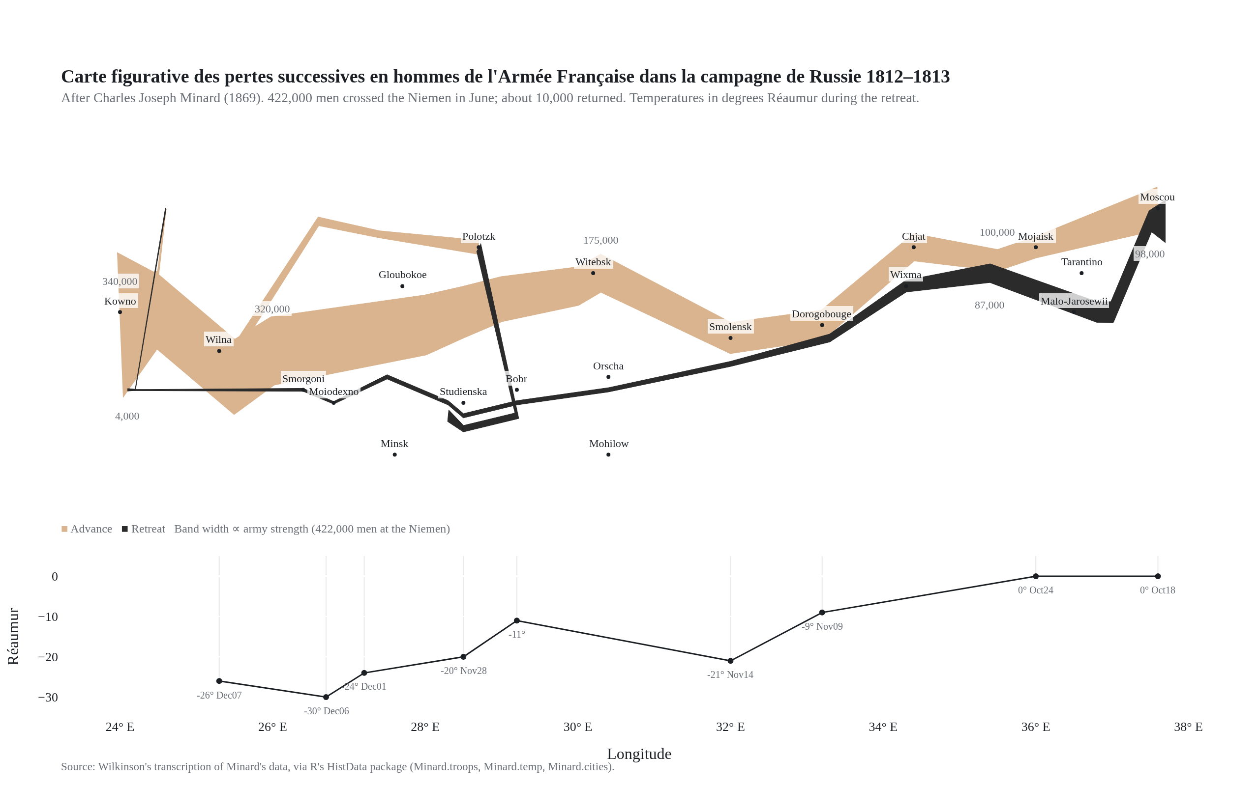
Minard's map

Python Code

"""Minard's map — Napoleon's Russian campaign of 1812, redrawn.

The most famous statistical graphic there is: army strength as band width,
advance and retreat as colour, cities along the route, and the retreat's
temperature in a second panel aligned on longitude. The tapering bands are
real polygons — offset curves computed from the troop counts and filled —
rather than lines of varying width.
"""
from pathlib import Path

from _shared import fetch_csv, save, base_layout, titles, INK, MUTED, GRID, SERIF

import numpy as np
import plotly.graph_objects as go
from plotly.subplots import make_subplots

CHART_NUM = 8
BASE = "https://vincentarelbundock.github.io/Rdatasets/csv/HistData/"
ADVANCE, RETREAT = "#d9b48f", "#2b2b2b"
LAT_PER_MAN = 0.7 / 422000   # band width in degrees of latitude per soldier
ASPECT = 1.7                 # degrees of longitude per degree of latitude on screen


def ribbon(x, y, w):
    """Polygon outline of a band along (x, y) with half-width w at each vertex.

    Normals are computed per segment and averaged at the joints (a mitre with
    its length clamped), so the band tapers smoothly and never spikes where
    the path doubles back.
    """
    pts = np.c_[np.asarray(x, float) * ASPECT, np.asarray(y, float)]  # screen-proportional space
    w = np.asarray(w, float)
    keep = np.r_[True, np.hypot(*np.diff(pts, axis=0).T) > 1e-9]        # drop repeated points
    pts, w = pts[keep], w[keep]
    seg = np.diff(pts, axis=0)
    seg_n = np.c_[-seg[:, 1], seg[:, 0]] / np.hypot(*seg.T)[:, None]
    vert_n = np.vstack([seg_n[:1], seg_n[:-1] + seg_n[1:], seg_n[-1:]])
    length = np.hypot(*vert_n.T)[:, None]
    vert_n = vert_n / np.where(length < 1e-9, 1, length)
    cos_half = np.clip(length[:, 0] / 2, 0.35, 1)       # mitre limit
    off = vert_n * (w / cos_half)[:, None]
    left, right = pts + off, pts - off
    poly = np.r_[left, right[::-1]]
    return np.c_[poly[:, 0] / ASPECT, poly[:, 1]]


def generate():
    troops = fetch_csv(BASE + "Minard.troops.csv")
    temp = fetch_csv(BASE + "Minard.temp.csv").sort_values("long")
    cities = fetch_csv(BASE + "Minard.cities.csv")

    fig = make_subplots(rows=2, cols=1, shared_xaxes=True, row_heights=[0.72, 0.28], vertical_spacing=0.04)

    for (group, direction), g in troops.groupby(["group", "direction"], sort=False):
        if len(g) < 2:
            continue
        poly = ribbon(g["long"], g["lat"], g["survivors"] * LAT_PER_MAN / 2)
        fig.add_trace(go.Scatter(
            x=poly[:, 0], y=poly[:, 1], mode="lines", fill="toself",
            fillcolor=ADVANCE if direction == "A" else RETREAT,
            line=dict(color=ADVANCE if direction == "A" else RETREAT, width=0.5),
            hoverinfo="skip", name=f"{'Advance' if direction == 'A' else 'Retreat'} (corps {group})",
        ), row=1, col=1)

    # Strength labels along the main army, above on the advance and below on the retreat.
    main = troops[troops["group"] == 1].reset_index(drop=True)
    halo = dict(bgcolor="rgba(255,255,255,0.78)", borderpad=1)  # keeps type legible over the dark band
    for idx in [0, 3, 9, 13, 17, 20, len(main) - 1]:
        p = main.iloc[idx]
        fig.add_annotation(x=p["long"], y=p["lat"], text=f"{int(p['survivors']):,}", showarrow=False,
                           yshift=(-26 - p["survivors"] * LAT_PER_MAN * 40) if p["direction"] == "R" else (22 + p["survivors"] * LAT_PER_MAN * 40),
                           font=dict(size=11, color=MUTED, family=SERIF), row=1, col=1, **halo)

    fig.add_trace(go.Scatter(x=cities["long"], y=cities["lat"], mode="markers", text=cities["city"],
                             marker=dict(size=4, color=INK), hoverinfo="text"), row=1, col=1)
    for _, c in cities.iterrows():
        fig.add_annotation(x=c["long"], y=c["lat"], text=c["city"], showarrow=False, yshift=12,
                           font=dict(size=11, color=INK, family=SERIF), row=1, col=1, **halo)

    fig.add_trace(go.Scatter(x=temp["long"], y=temp["temp"], mode="lines+markers", line=dict(color=INK, width=1.5),
                             marker=dict(size=6, color=INK), hovertemplate="%{y} °R<extra></extra>"), row=2, col=1)
    for _, t in temp.iterrows():
        lab = f"{int(t['temp'])}°" + (f" {t['date']}" if isinstance(t["date"], str) else "")
        fig.add_annotation(x=t["long"], y=t["temp"], text=lab, showarrow=False, yshift=-14,
                           font=dict(size=10, color=MUTED, family=SERIF), row=2, col=1)
        fig.add_shape(type="line", x0=t["long"], x1=t["long"], y0=t["temp"], y1=5, line=dict(color=GRID, width=1), row=2, col=1, layer="below")

    fig.update_layout(**base_layout(font=dict(family=SERIF, size=13, color=INK), margin=dict(l=60, r=40, t=120, b=70)))
    fig.update_xaxes(showgrid=False, range=[23.5, 38.5], row=1, col=1)
    fig.update_yaxes(showgrid=False, showticklabels=False, range=[53.4, 56.4], row=1, col=1, scaleanchor="x", scaleratio=ASPECT)
    fig.update_xaxes(showgrid=False, ticksuffix="° E", dtick=2, title_text="Longitude", row=2, col=1)
    fig.update_yaxes(range=[-35, 5], tickvals=[0, -10, -20, -30], ticksuffix="°", title_text="Réaumur", showgrid=True, row=2, col=1)
    fig.add_annotation(x=0.0, y=0.30, xref="paper", yref="paper", xanchor="left",
                       text=f"<span style='color:{ADVANCE}'>■</span> Advance   <span style='color:{RETREAT}'>■</span> Retreat   Band width ∝ army strength (422,000 men at the Niemen)",
                       showarrow=False, font=dict(size=12, color=MUTED, family=SERIF))
    titles(fig, "Carte figurative des pertes successives en hommes de l'Armée Française dans la campagne de Russie 1812–1813",
           "After Charles Joseph Minard (1869). 422,000 men crossed the Niemen in June; about 10,000 returned. Temperatures in degrees Réaumur during the retreat.",
           "Source: Wilkinson's transcription of Minard's data, via R's HistData package (Minard.troops, Minard.temp, Minard.cities).", size=19)
    save(CHART_NUM, fig)

Made with Plotly