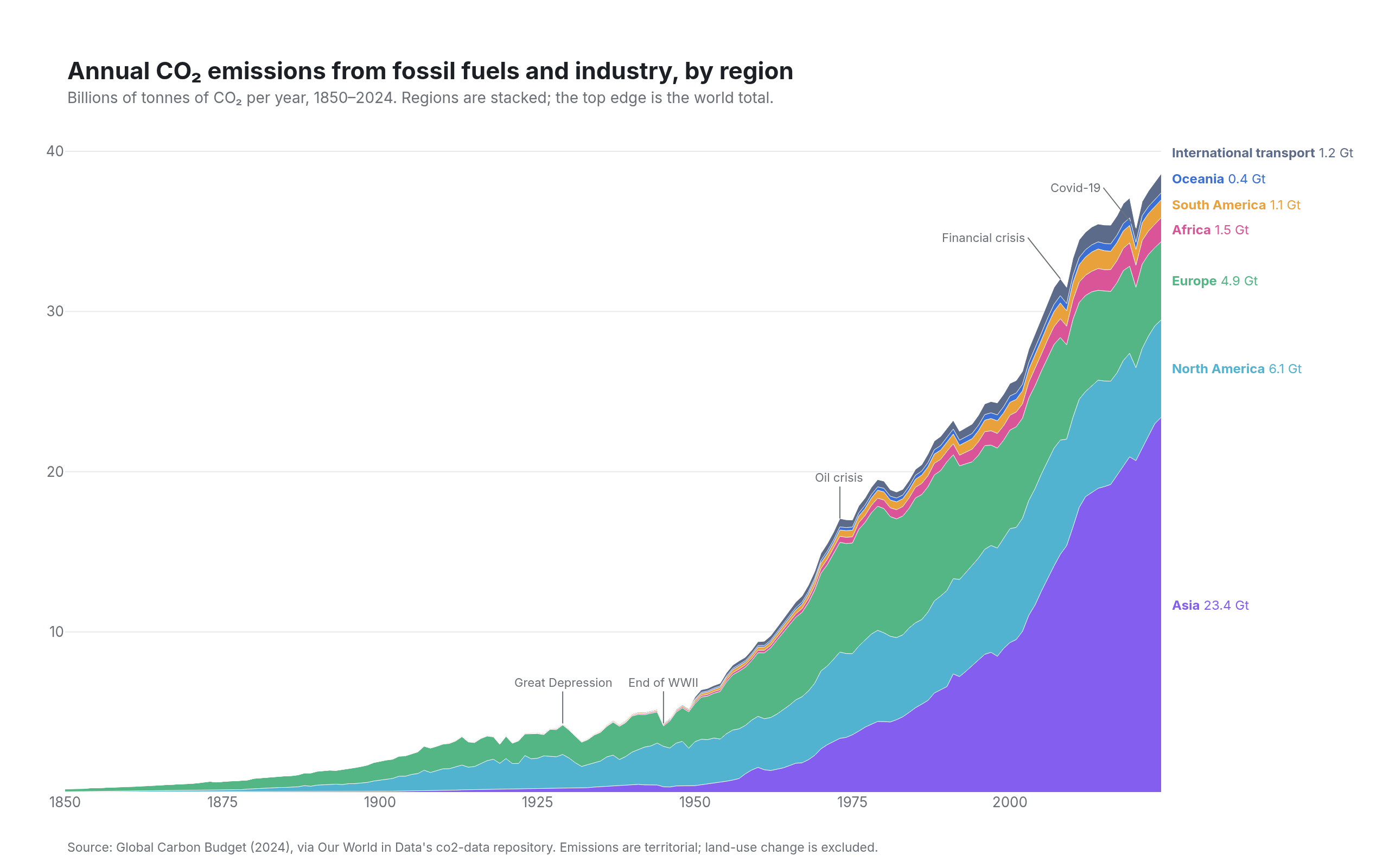
Stacked area with direct labels

Python Code

"""Stacked area with direct labels — CO₂ emissions by world region since 1850.

The Our World in Data treatment: regions stacked from largest to smallest,
labelled at the right edge where the eye lands, with the axis tucked away
and a few dated events pinned to the top of the stack.
"""
from pathlib import Path

from _shared import fetch_csv, save, base_layout, titles, INK, MUTED, FAINT, GRID, VIOLET, TEAL, GREEN, PINK, ORANGE, BLUE, SLATE

import numpy as np
import plotly.graph_objects as go

CHART_NUM = 14
URL = "https://raw.githubusercontent.com/owid/co2-data/master/owid-co2-data.csv"
REGIONS = [("Asia", VIOLET), ("North America", TEAL), ("Europe", GREEN), ("Africa", PINK),
           ("South America", ORANGE), ("Oceania", BLUE), ("International transport", SLATE)]
EVENTS = [(1929, "Great Depression"), (1945, "End of WWII"), (1973, "Oil crisis"), (2008, "Financial crisis"), (2020, "Covid-19")]


def generate():
    df = fetch_csv(URL, usecols=["country", "year", "co2"])
    df = df[df["country"].isin([r for r, _ in REGIONS] + ["World"]) & (df["year"] >= 1850)]
    wide = df.pivot(index="year", columns="country", values="co2").fillna(0) / 1000  # Mt → Gt
    # OWID's regions exclude international aviation and shipping; the remainder against the world total is that.
    wide["International transport"] = (wide["World"] - wide[[r for r, _ in REGIONS if r != "International transport"]].sum(axis=1)).clip(lower=0)
    wide = wide.drop(columns="World")
    order = [r for r, _ in REGIONS]
    colors = dict(REGIONS)
    fig = go.Figure()
    for r in order:
        fig.add_trace(go.Scatter(x=wide.index, y=wide[r], mode="lines", name=r, stackgroup="one",
                                 line=dict(width=0.5, color="white"), fillcolor=colors[r],
                                 hovertemplate="%{x}: %{y:.2f} Gt<extra>" + r + "</extra>"))
    # Direct labels at the right edge, at the vertical middle of each band in the last year.
    last = wide.iloc[-1]
    cum = 0
    labels = []
    for r in order:
        mid = cum + last[r] / 2
        cum += last[r]
        labels.append((r, mid, last[r]))
    # Nudge the small ones apart.
    pos = np.array([m for _, m, _ in labels])
    for _ in range(100):
        for i in range(len(pos) - 1):
            if pos[i + 1] - pos[i] < 1.6:
                pos[i + 1] = pos[i] + 1.6
    for (r, _, v), y in zip(labels, pos):
        fig.add_annotation(x=wide.index[-1], y=y, text=f"<b>{r}</b> {v:.1f} Gt", showarrow=False, xanchor="left", xshift=8,
                           font=dict(size=12, color=colors[r]))
    total = wide.sum(axis=1)
    for yr, text in EVENTS:
        fig.add_annotation(x=yr, y=total.loc[yr], text=text, showarrow=True, arrowhead=0, arrowwidth=1, arrowcolor=MUTED,
                           ax=-30 if yr >= 2000 else 0, ay=-38, xanchor="right" if yr >= 2000 else "center", font=dict(size=11, color=MUTED))

    fig.update_layout(**base_layout(margin=dict(l=60, r=210, t=110, b=70)))
    fig.update_xaxes(range=[1850, wide.index[-1]], dtick=25, showgrid=False)
    fig.update_yaxes(range=[0, 42], tickvals=[10, 20, 30, 40], ticksuffix=" Gt", title_text=None)
    titles(fig, "Annual CO₂ emissions from fossil fuels and industry, by region",
           f"Billions of tonnes of CO₂ per year, 1850–{wide.index[-1]}. Regions are stacked; the top edge is the world total.",
           "Source: Global Carbon Budget (2024), via Our World in Data's co2-data repository. Emissions are territorial; land-use change is excluded.")
    save(CHART_NUM, fig)

Made with Plotly