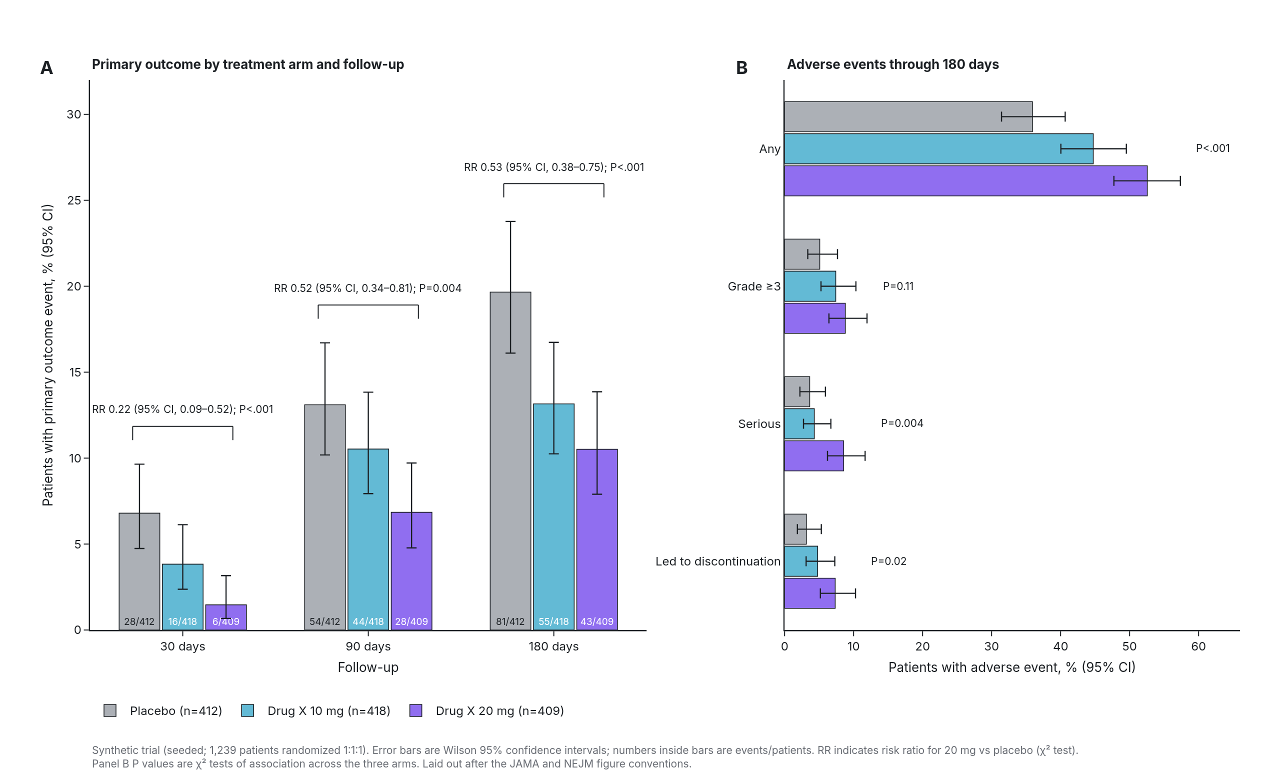
Clinical bar chart

Python Code

"""Clinical bar chart — event rates by treatment arm, the way a medical journal sets them.

Two lettered panels in the JAMA/NEJM idiom: grouped bars of the primary
outcome by arm and follow-up with Wilson 95% confidence intervals, the
risk ratio and its interval written over each comparison bracket, and a
second panel of adverse events by grade. Group sizes live in the axis
labels, exact P values in the brackets, and nothing is drawn that a
reviewer would ask to remove.
"""
from pathlib import Path

from _shared import save, base_layout, panel_label, INK, MUTED, FAINT, VIOLET, TEAL, hex_to_rgba

import numpy as np
import plotly.graph_objects as go
from plotly.subplots import make_subplots
from scipy import stats

CHART_NUM = 32
rng = np.random.default_rng(2024)
ARMS = [("Placebo", 412, FAINT), ("Drug X 10 mg", 418, TEAL), ("Drug X 20 mg", 409, VIOLET)]
TIMES = ["30 days", "90 days", "180 days"]
TRUE_RATE = {"Placebo": [0.062, 0.128, 0.191], "Drug X 10 mg": [0.048, 0.093, 0.142], "Drug X 20 mg": [0.036, 0.071, 0.104]}
GRADES = ["Any", "Grade ≥3", "Serious", "Led to discontinuation"]
TRUE_AE = {"Placebo": [0.38, 0.061, 0.043, 0.024], "Drug X 10 mg": [0.44, 0.079, 0.051, 0.037], "Drug X 20 mg": [0.51, 0.104, 0.064, 0.058]}
AX = dict(showgrid=False, showline=True, linecolor=INK, linewidth=1.2, ticks="outside", tickcolor=INK, ticklen=5,
          tickfont=dict(size=12, color=INK), title=dict(font=dict(size=13, color=INK), standoff=10), zeroline=False)


def wilson(k, n, z=1.96):
    p = k / n
    d = 1 + z ** 2 / n
    c = (p + z ** 2 / (2 * n)) / d
    h = z * np.sqrt(p * (1 - p) / n + z ** 2 / (4 * n ** 2)) / d
    return c - h, c + h


def fmt_p(p):
    return "P<.001" if p < 0.001 else f"P={p:.3f}" if p < 0.01 else f"P={p:.2f}"


def generate():
    events = {a: [rng.binomial(n, r) for r in TRUE_RATE[a]] for a, n, _ in ARMS}
    aes = {a: [rng.binomial(n, r) for r in TRUE_AE[a]] for a, n, _ in ARMS}
    fig = make_subplots(rows=1, cols=2, horizontal_spacing=0.12, column_widths=[0.55, 0.45])

    # A: primary outcome by follow-up, grouped by arm.
    for arm, n, color in ARMS:
        k = np.array(events[arm]); p = k / n * 100
        lo, hi = wilson(k, n)
        fig.add_trace(go.Bar(
            x=TIMES, y=p, name=f"{arm} (n={n})", marker=dict(color=hex_to_rgba(color, 0.9), line=dict(color=INK, width=0.8)),
            error_y=dict(type="data", symmetric=False, array=hi * 100 - p, arrayminus=p - lo * 100, color=INK, thickness=1.2, width=5),
            text=[f"{ki}/{n}" for ki in k], textposition="inside", insidetextanchor="start", textangle=0, constraintext="none",
            textfont=dict(size=9.5, color="white" if color != FAINT else INK),
            hovertemplate="%{x}: %{y:.1f}% (95% CI %{customdata[0]:.1f}–%{customdata[1]:.1f})<extra>" + arm + "</extra>",
            customdata=np.c_[lo * 100, hi * 100], legendgroup=arm,
        ), row=1, col=1)
    # Brackets: 20 mg vs placebo at each follow-up, with RR (95% CI) and P.
    gap = 0.27
    for i, t in enumerate(TIMES):
        k0, n0 = events["Placebo"][i], ARMS[0][1]
        k2, n2 = events["Drug X 20 mg"][i], ARMS[2][1]
        rr = (k2 / n2) / (k0 / n0)
        se = np.sqrt(1 / k2 - 1 / n2 + 1 / k0 - 1 / n0)
        lo, hi = np.exp(np.log(rr) - 1.96 * se), np.exp(np.log(rr) + 1.96 * se)
        p = stats.chi2_contingency([[k0, n0 - k0], [k2, n2 - k2]])[1]
        top = max(wilson(k0, n0)[1], wilson(k2, n2)[1]) * 100 + 2.2
        for x0, x1, y0, y1 in [(i - gap, i + gap, top, top), (i - gap, i - gap, top - 0.8, top), (i + gap, i + gap, top - 0.8, top)]:
            fig.add_shape(type="line", x0=x0, x1=x1, y0=y0, y1=y1, xref="x", yref="y", line=dict(color=INK, width=1))
        fig.add_annotation(x=i, y=top, xref="x", yref="y", yshift=8, showarrow=False, font=dict(size=10.5, color=INK), yanchor="bottom",
                           text=f"RR {rr:.2f} (95% CI, {lo:.2f}–{hi:.2f}); {fmt_p(p)}")

    # B: adverse events by grade, horizontal grouped bars.
    for arm, n, color in ARMS:
        k = np.array(aes[arm]); p = k / n * 100
        lo, hi = wilson(k, n)
        fig.add_trace(go.Bar(
            y=GRADES, x=p, orientation="h", name=f"{arm} (n={n})", marker=dict(color=hex_to_rgba(color, 0.9), line=dict(color=INK, width=0.8)),
            error_x=dict(type="data", symmetric=False, array=hi * 100 - p, arrayminus=p - lo * 100, color=INK, thickness=1.2, width=5),
            showlegend=False, legendgroup=arm,
            hovertemplate="%{y}: %{x:.1f}% (95% CI %{customdata[0]:.1f}–%{customdata[1]:.1f})<extra>" + arm + "</extra>",
            customdata=np.c_[lo * 100, hi * 100],
        ), row=1, col=2)
    # Cochran–Armitage-style trend test across doses, one per grade, written at the row's right.
    for j, g in enumerate(GRADES):
        ks = [aes[a][j] for a, _, _ in ARMS]; ns = [n for _, n, _ in ARMS]
        table = [[k, n - k] for k, n in zip(ks, ns)]
        p = stats.chi2_contingency(table)[1]
        fig.add_annotation(x=max(wilson(k, n)[1] for k, n in zip(ks, ns)) * 100 + 2, y=g, xref="x2", yref="y2", xanchor="left", showarrow=False,
                           text=fmt_p(p), font=dict(size=10.5, color=INK))

    fig.update_layout(**base_layout(barmode="group", bargap=0.3, bargroupgap=0.06, margin=dict(l=90, r=40, t=80, b=150), showlegend=True,
                                    legend=dict(orientation="h", x=0.0, y=-0.12, xanchor="left", yanchor="top", font=dict(size=12, color=INK), traceorder="normal")))
    fig.update_xaxes(**AX, row=1, col=1, title_text="Follow-up")
    fig.update_yaxes(**AX, row=1, col=1, title_text="Patients with primary outcome event, % (95% CI)", range=[0, 32], dtick=5, ticksuffix="")
    fig.update_xaxes(**AX, row=1, col=2, title_text="Patients with adverse event, % (95% CI)", range=[0, 66], dtick=10)
    fig.update_yaxes(**{**AX, "ticklen": 0}, row=1, col=2, autorange="reversed")
    panel_label(fig, "A", x=fig.layout.xaxis.domain[0] - 0.03, y=1.0, size=18)
    panel_label(fig, "B", x=fig.layout.xaxis2.domain[0] - 0.03, y=1.0, size=18)
    fig.add_annotation(x=fig.layout.xaxis.domain[0], y=1.0, xref="paper", yref="paper", xanchor="left", yanchor="bottom", yshift=6, showarrow=False,
                       text="<b>Primary outcome by treatment arm and follow-up</b>", font=dict(size=13, color=INK))
    fig.add_annotation(x=fig.layout.xaxis2.domain[0], y=1.0, xref="paper", yref="paper", xanchor="left", yanchor="bottom", yshift=6, showarrow=False,
                       text="<b>Adverse events through 180 days</b>", font=dict(size=13, color=INK))
    fig.add_annotation(x=0, y=0, xref="paper", yref="paper", xanchor="left", yanchor="top", yshift=-112, showarrow=False, align="left",
                       font=dict(size=10.5, color=MUTED),
                       text="Synthetic trial (seeded; 1,239 patients randomized 1:1:1). Error bars are Wilson 95% confidence intervals; numbers inside bars are events/patients. "
                            "RR indicates risk ratio for 20 mg vs placebo (χ² test).<br>Panel B P values are χ² tests of association across the three arms. "
                            "Laid out after the JAMA and NEJM figure conventions.")
    save(CHART_NUM, fig, width=1280, height=780)

Made with Plotly