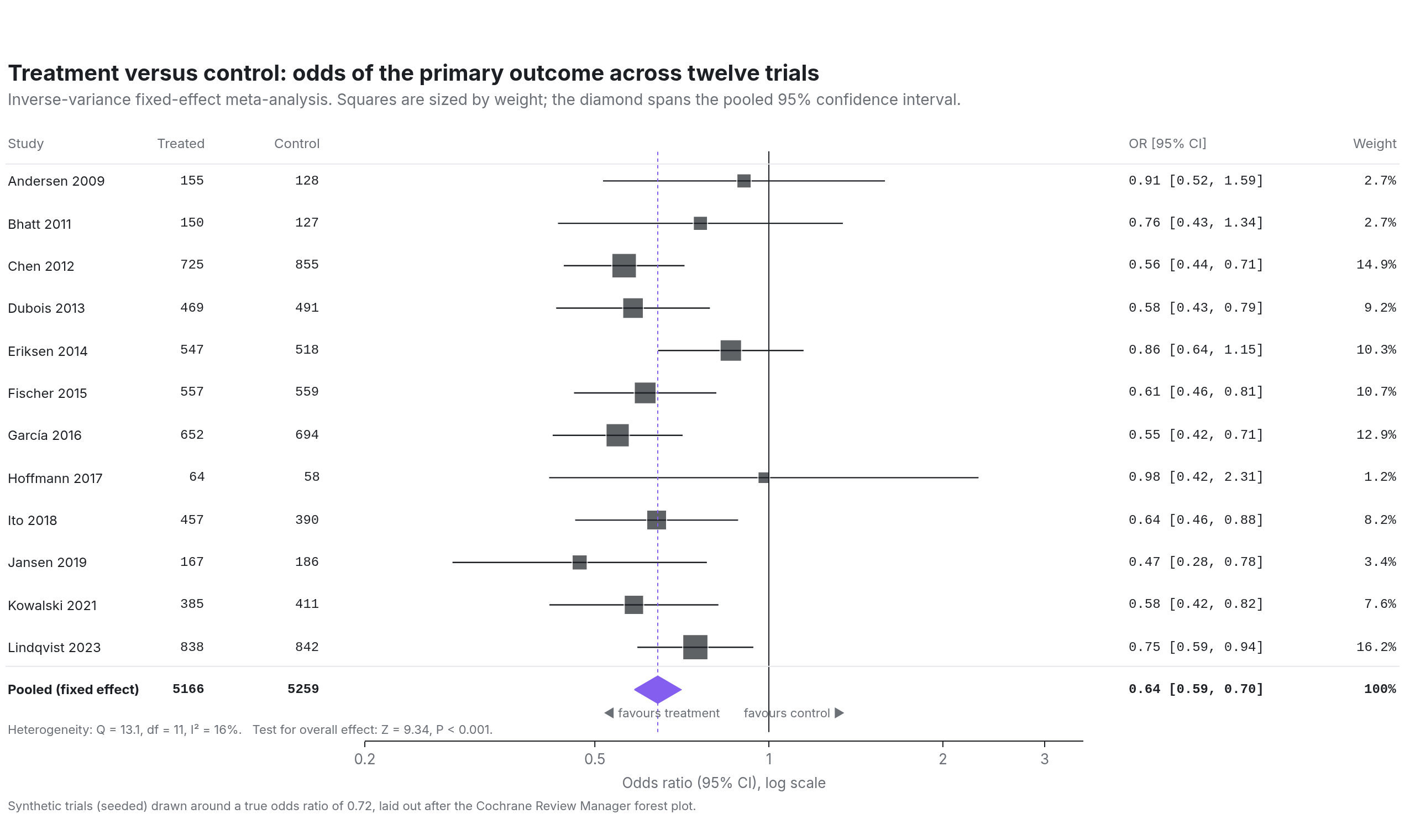
a meta-analysis of twelve trials, in the Cochrane layout

Python Code

"""Forest plot — a meta-analysis of twelve trials, in the Cochrane layout.

The evidence-synthesis figure: one row per study with its odds ratio and
confidence interval, squares sized by weight, a diamond for the pooled
estimate, a log axis through 1, and the numbers themselves typeset in
columns either side of the plot so it reads as a table and a chart at once.
"""
from pathlib import Path

from _shared import save, base_layout, INK, MUTED, FAINT, GRID, VIOLET, MONO, hex_to_rgba

import numpy as np
import plotly.graph_objects as go

CHART_NUM = 24
rng = np.random.default_rng(11)
STUDIES = ["Andersen 2009", "Bhatt 2011", "Chen 2012", "Dubois 2013", "Eriksen 2014", "Fischer 2015",
           "García 2016", "Hoffmann 2017", "Ito 2018", "Jansen 2019", "Kowalski 2021", "Lindqvist 2023"]


def generate():
    n_t = rng.integers(40, 900, len(STUDIES)); n_c = (n_t * rng.uniform(0.8, 1.2, len(STUDIES))).astype(int)
    true_or = 0.72
    log_or = np.log(true_or) + rng.normal(0, 0.18, len(STUDIES))
    se = np.sqrt(1 / (n_t * 0.15) + 1 / (n_c * 0.2))
    log_or += rng.normal(0, se)
    lo, hi = np.exp(log_or - 1.96 * se), np.exp(log_or + 1.96 * se)
    w = 1 / se ** 2; w_pct = w / w.sum() * 100
    pooled = (w * log_or).sum() / w.sum(); pooled_se = np.sqrt(1 / w.sum())
    p_lo, p_hi = np.exp(pooled - 1.96 * pooled_se), np.exp(pooled + 1.96 * pooled_se)
    q = (w * (log_or - pooled) ** 2).sum(); i2 = max(0, (q - (len(STUDIES) - 1)) / q) * 100
    z = pooled / pooled_se

    rows = len(STUDIES)
    y = np.arange(rows)[::-1] + 1      # study rows from top; pooled at y = 0
    fig = go.Figure()
    fig.add_shape(type="line", x0=1, x1=1, y0=-1, y1=rows + 0.7, line=dict(color=INK, width=1))
    fig.add_shape(type="line", x0=np.exp(pooled), x1=np.exp(pooled), y0=-1, y1=rows + 0.7, line=dict(color=VIOLET, width=1, dash="dot"))
    for i in range(rows):
        fig.add_trace(go.Scatter(x=[lo[i], hi[i]], y=[y[i], y[i]], mode="lines", line=dict(color=INK, width=1.2), hoverinfo="skip"))
    fig.add_trace(go.Scatter(x=np.exp(log_or), y=y, mode="markers", marker=dict(symbol="square", size=6 + np.sqrt(w_pct) * 4.2, color=INK),
                             text=STUDIES, hovertemplate="%{text}: OR %{x:.2f}<extra></extra>"))
    # Pooled diamond: centre at the estimate, tips at the CI bounds.
    fig.add_trace(go.Scatter(x=[p_lo, np.exp(pooled), p_hi, np.exp(pooled), p_lo], y=[0, 0.32, 0, -0.32, 0], fill="toself",
                             fillcolor=VIOLET, line=dict(color=VIOLET, width=1), mode="lines", hovertemplate=f"Pooled OR {np.exp(pooled):.2f}<extra></extra>"))
    # Table columns in paper coordinates on either side of the plot.
    fig.update_layout(**base_layout(margin=dict(l=330, r=300, t=110, b=90), font=dict(size=12)))
    fig.update_xaxes(type="log", range=[np.log10(0.2), np.log10(3.5)], tickvals=[0.2, 0.5, 1, 2, 3], ticktext=["0.2", "0.5", "1", "2", "3"],
                     showgrid=False, showline=True, linecolor=INK, ticks="outside", tickcolor=INK, title_text="Odds ratio (95% CI), log scale")
    fig.update_yaxes(visible=False, range=[-1.2, rows + 1.4])

    def col(x, ytxt, text, anchor="left", bold=False, color=INK, mono=False):
        fig.add_annotation(x=x, y=ytxt, xref="paper", yref="y", text=f"<b>{text}</b>" if bold else text, showarrow=False,
                           xanchor=anchor, font=dict(size=12, color=color, family=MONO if mono else None))
    for i, s in enumerate(STUDIES):
        col(-0.50, y[i], s); col(-0.22, y[i], f"{n_t[i]}", "right", mono=True); col(-0.06, y[i], f"{n_c[i]}", "right", mono=True)
        col(1.06, y[i], f"{np.exp(log_or[i]):.2f} [{lo[i]:.2f}, {hi[i]:.2f}]", mono=True); col(1.44, y[i], f"{w_pct[i]:.1f}%", "right", mono=True)
    col(-0.50, 0, "Pooled (fixed effect)", bold=True); col(-0.22, 0, f"{n_t.sum()}", "right", bold=True, mono=True); col(-0.06, 0, f"{n_c.sum()}", "right", bold=True, mono=True)
    col(1.06, 0, f"{np.exp(pooled):.2f} [{p_lo:.2f}, {p_hi:.2f}]", bold=True, mono=True); col(1.44, 0, "100%", "right", bold=True, mono=True)
    hdr = rows + 0.9
    for x, t, a in [(-0.50, "Study", "left"), (-0.22, "Treated", "right"), (-0.06, "Control", "right"), (1.06, "OR [95% CI]", "left"), (1.44, "Weight", "right")]:
        col(x, hdr, t, a, color=MUTED)
    fig.add_shape(type="line", x0=-0.50, x1=1.44, xref="paper", y0=hdr - 0.5, y1=hdr - 0.5, yref="y", line=dict(color=GRID, width=1))
    fig.add_shape(type="line", x0=-0.50, x1=1.44, xref="paper", y0=0.55, y1=0.55, yref="y", line=dict(color=GRID, width=1))
    fig.add_annotation(x=-0.50, y=-0.95, xref="paper", yref="y", xanchor="left", showarrow=False, font=dict(size=11, color=MUTED), align="left",
                       text=f"Heterogeneity: Q = {q:.1f}, df = {rows - 1}, I² = {i2:.0f}%.   Test for overall effect: Z = {abs(z):.2f}, P {'< 0.001' if abs(z) > 3.29 else '= ' + f'{2 * (1 - 0.5 * (1 + np.math.erf(abs(z) / np.sqrt(2)))):.3f}'}.")
    fig.add_annotation(x=0.5, y=-0.55, xref="paper", yref="y", showarrow=False, font=dict(size=11, color=MUTED),
                       text="◀ favours treatment       favours control ▶")
    fig.add_annotation(x=-0.50, y=1.0, xref="paper", yref="paper", xanchor="left", yanchor="bottom", yshift=30, showarrow=False,
                       text="<b>Treatment versus control: odds of the primary outcome across twelve trials</b>", font=dict(size=20, color=INK))
    fig.add_annotation(x=-0.50, y=1.0, xref="paper", yref="paper", xanchor="left", yanchor="bottom", yshift=10, showarrow=False,
                       text="Inverse-variance fixed-effect meta-analysis. Squares are sized by weight; the diamond spans the pooled 95% confidence interval.", font=dict(size=14, color=MUTED))
    fig.add_annotation(x=-0.50, y=0, xref="paper", yref="paper", xanchor="left", yanchor="top", yshift=-50, showarrow=False,
                       text="Synthetic trials (seeded) drawn around a true odds ratio of 0.72, laid out after the Cochrane Review Manager forest plot.", font=dict(size=11, color=MUTED))
    save(CHART_NUM, fig, width=1280, height=760)

Made with Plotly