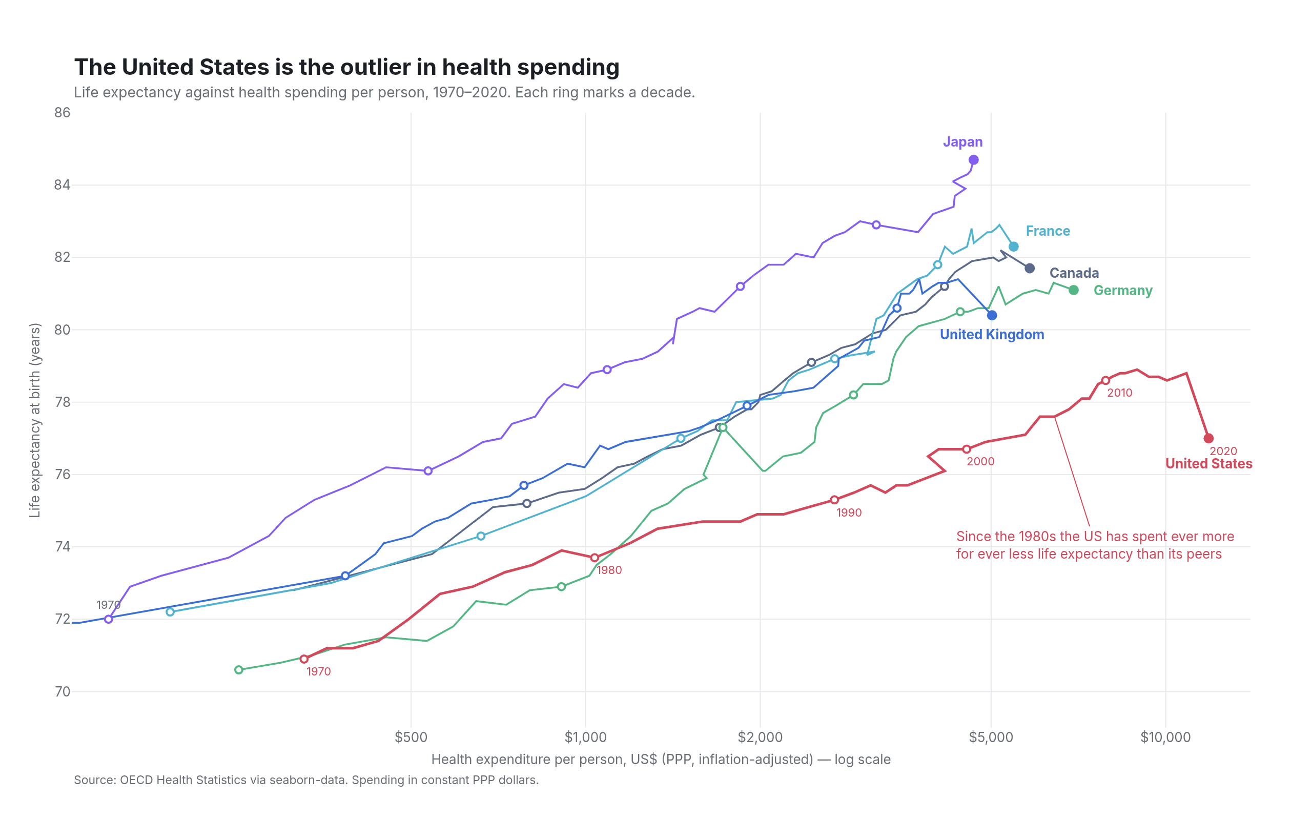
Connected scatterplot

Python Code

"""Connected scatterplot — health spending vs life expectancy, 1970–2020.

The Our World in Data classic. Each country is a path through time on a log
x axis, with the decades ticked along the path, the endpoints labelled
directly, and the outlier drawn in the only saturated colour.
"""
from pathlib import Path

from _shared import fetch_csv, save, base_layout, titles, INK, MUTED, FAINT, GRID, RED, SLATE, TEAL, VIOLET, GREEN, BLUE, hex_to_rgba

import numpy as np
import plotly.graph_objects as go

CHART_NUM = 4
URL = "https://raw.githubusercontent.com/mwaskom/seaborn-data/master/healthexp.csv"
COLORS = {"USA": RED, "Japan": VIOLET, "France": TEAL, "Germany": GREEN, "Great Britain": BLUE, "Canada": SLATE}
LABEL = {"USA": "United States", "Great Britain": "United Kingdom"}
# (dx, dy) pixel offsets for the endpoint labels, tuned by hand.
END_OFFSET = {"USA": (0, -24), "Japan": (-10, 18), "France": (34, 16), "Germany": (48, 0),
              "Great Britain": (0, -18), "Canada": (44, -4)}


def generate():
    df = fetch_csv(URL).sort_values(["Country", "Year"])
    fig = go.Figure()
    for country, g in df.groupby("Country"):
        c = COLORS[country]
        x, y = g["Spending_USD"], g["Life_Expectancy"]
        fig.add_trace(go.Scatter(
            x=x, y=y, mode="lines", name=country,
            line=dict(color=c, width=2.5 if country == "USA" else 1.8),
            hovertemplate="%{text}<br>$%{x:,.0f} · %{y:.1f} yrs<extra></extra>", text=[f"{country} {yr}" for yr in g["Year"]],
        ))
        decades = g[g["Year"] % 10 == 0]
        fig.add_trace(go.Scatter(
            x=decades["Spending_USD"], y=decades["Life_Expectancy"], mode="markers",
            marker=dict(size=7, color="white", line=dict(color=c, width=2)),
            hoverinfo="skip", showlegend=False,
        ))
        first, last = g.iloc[0], g.iloc[-1]
        fig.add_trace(go.Scatter(x=[last["Spending_USD"]], y=[last["Life_Expectancy"]], mode="markers",
                                 marker=dict(size=10, color=c), hoverinfo="skip"))
        dx, dy = END_OFFSET[country]
        fig.add_annotation(x=np.log10(last["Spending_USD"]), y=last["Life_Expectancy"], text=f"<b>{LABEL.get(country, country)}</b>",
                           showarrow=False, xshift=dx, yshift=dy, font=dict(size=13, color=c))
        if country == "USA":
            for _, row in decades.iterrows():
                fig.add_annotation(x=np.log10(row["Spending_USD"]), y=row["Life_Expectancy"], text=str(int(row["Year"])),
                                   showarrow=False, xshift=14, yshift=-12, font=dict(size=11, color=c))
    fig.add_annotation(x=np.log10(df[df.Country == "Japan"].iloc[0]["Spending_USD"]), y=df[df.Country == "Japan"].iloc[0]["Life_Expectancy"],
                       text="1970", showarrow=False, yshift=14, font=dict(size=11, color=MUTED))

    us2005 = df[(df["Country"] == "USA") & (df["Year"] == 2005)].iloc[0]
    fig.add_annotation(x=np.log10(us2005["Spending_USD"]), y=us2005["Life_Expectancy"],
                       text="Since the 1980s the US has spent ever more<br>for ever less life expectancy than its peers",
                       showarrow=True, arrowhead=0, arrowcolor=RED, arrowwidth=1, ax=40, ay=125,
                       font=dict(size=13, color=RED), align="left", xanchor="center")

    fig.update_layout(**base_layout(margin=dict(l=70, r=60, t=110, b=90)))
    fig.update_xaxes(type="log", title_text="Health expenditure per person, US$ (PPP, inflation-adjusted) — log scale",
                     tickvals=[500, 1000, 2000, 5000, 10000], ticktext=["$500", "$1,000", "$2,000", "$5,000", "$10,000"],
                     range=[np.log10(130), np.log10(14000)])
    fig.update_yaxes(title_text="Life expectancy at birth (years)", range=[69, 86], dtick=2)

    titles(fig, "The United States is the outlier in health spending",
           "Life expectancy against health spending per person, 1970–2020. Each ring marks a decade.",
           "Source: OECD Health Statistics via seaborn-data. Spending in constant PPP dollars.")
    save(CHART_NUM, fig)

Made with Plotly