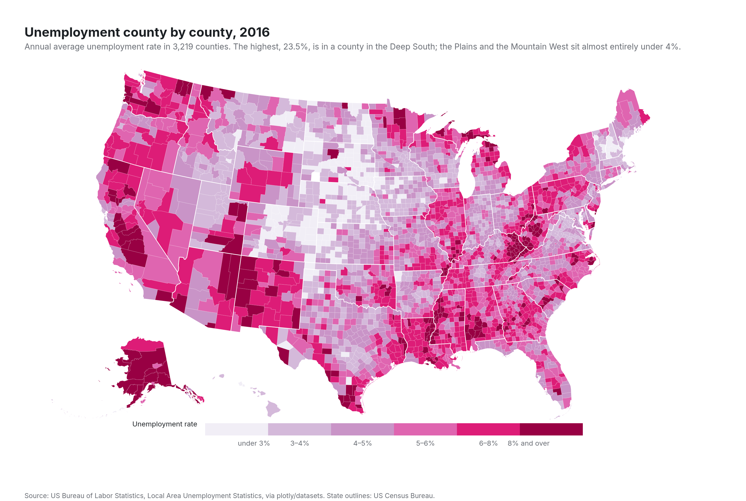
County choropleth

Python Code

"""County choropleth — US unemployment rate by county, 2016.

A print map: Albers USA projection, no frame or graticule, states outlined
in white, counties binned into six classes on a sequential ramp, and a
hand-built swatch legend along the bottom instead of a continuous colourbar.
"""
from pathlib import Path

from _shared import fetch_csv, fetch_json, save, base_layout, titles, INK, MUTED, FAINT

import numpy as np
import plotly.graph_objects as go

CHART_NUM = 11
CSV = "https://raw.githubusercontent.com/plotly/datasets/master/fips-unemp-16.csv"
GEO = "https://raw.githubusercontent.com/plotly/datasets/master/geojson-counties-fips.json"
STATES = "https://raw.githubusercontent.com/PublicaMundi/MappingAPI/master/data/geojson/us-states.json"
BINS = [0, 3, 4, 5, 6, 8, 100]
LABELS = ["under 3%", "3–4%", "4–5%", "5–6%", "6–8%", "8% and over"]
RAMP = ["#f1eef6", "#d4b9da", "#c994c7", "#df65b0", "#dd1c77", "#980043"]  # ColorBrewer PuRd


def generate():
    df = fetch_csv(CSV, dtype={"fips": str})
    counties = fetch_json(GEO)
    cls = np.digitize(df["unemp"], BINS[1:-1])  # 0..5
    # A stepped colorscale so the continuous colour axis renders discrete classes.
    steps = []
    for i, c in enumerate(RAMP):
        steps += [[i / 6, c], [(i + 1) / 6, c]]
    fig = go.Figure(go.Choropleth(
        geojson=counties, locations=df["fips"], z=cls, zmin=-0.5, zmax=5.5, colorscale=steps,
        marker=dict(line=dict(width=0.15, color="white")), showscale=False,
        customdata=df["unemp"], hovertemplate="FIPS %{location}: %{customdata:.1f}%<extra></extra>",
    ))
    # State borders drawn on top of the counties as one None-gapped line trace.
    lons, lats = [], []
    for feat in fetch_json(STATES)["features"]:
        geom = feat["geometry"]
        polys = geom["coordinates"] if geom["type"] == "MultiPolygon" else [geom["coordinates"]]
        for poly in polys:
            for ring in poly:
                lons += [pt[0] for pt in ring] + [None]
                lats += [pt[1] for pt in ring] + [None]
    fig.add_trace(go.Scattergeo(lon=lons, lat=lats, mode="lines", line=dict(color="white", width=1.1), hoverinfo="skip"))
    fig.update_geos(scope="usa", projection_type="albers usa", showlakes=False, showland=False, showcoastlines=False,
                    showframe=False, showsubunits=False, bgcolor="white",
                    domain=dict(x=[0, 1], y=[0.1, 1.0]))
    fig.update_layout(**base_layout(margin=dict(l=40, r=40, t=100, b=60)))
    # Swatch legend, built from shapes so it can sit exactly where a print legend would.
    x0, w, yb = 0.26, 0.09, 0.075
    for i, (c, lab) in enumerate(zip(RAMP, LABELS)):
        fig.add_shape(type="rect", xref="paper", yref="paper", x0=x0 + i * w, x1=x0 + (i + 1) * w, y0=yb, y1=yb + 0.03,
                      fillcolor=c, line=dict(width=0))
        fig.add_annotation(x=x0 + (i + 0.5) * w, y=yb - 0.005, xref="paper", yref="paper", text=lab, showarrow=False,
                           yanchor="top", font=dict(size=12, color=MUTED))
    fig.add_annotation(x=x0 - 0.01, y=yb + 0.015, xref="paper", yref="paper", text="Unemployment rate", showarrow=False,
                       xanchor="right", font=dict(size=12, color=INK))
    hi = df.loc[df["unemp"].idxmax()]
    titles(fig, "Unemployment county by county, 2016",
           f"Annual average unemployment rate in {len(df):,} counties. The highest, {hi['unemp']:.1f}%, is in a county in the Deep South; "
           "the Plains and the Mountain West sit almost entirely under 4%.",
           "Source: US Bureau of Labor Statistics, Local Area Unemployment Statistics, via plotly/datasets. State outlines: US Census Bureau.")
    save(CHART_NUM, fig, width=1280, height=860)

Made with Plotly