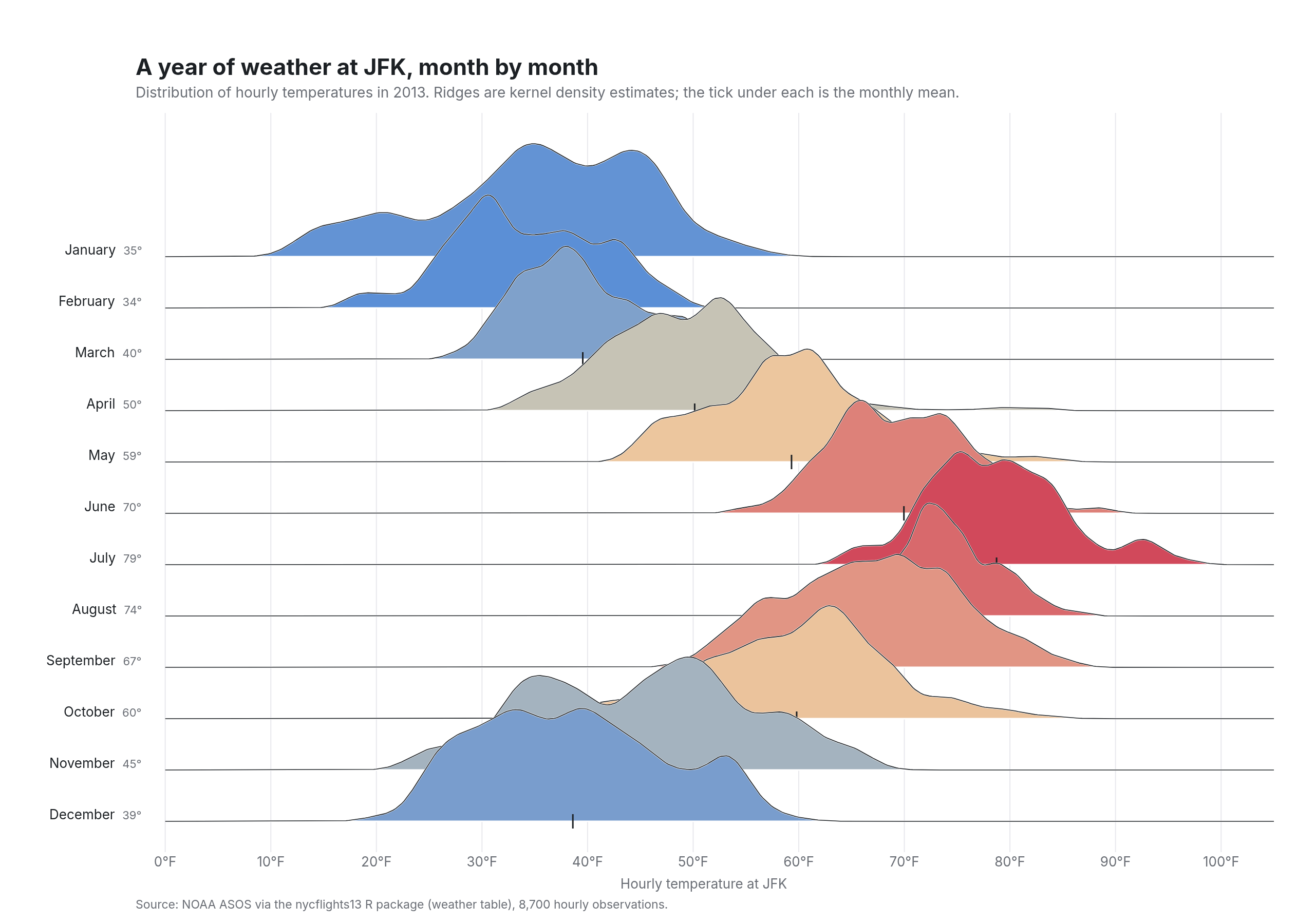
Ridgeline plot

Python Code

"""Ridgeline plot — a year of New York hourly temperatures, one ridge per month.

Twelve kernel density estimates stacked with a deliberate overlap, filled
on a temperature-coloured ramp, with the months set down the left margin
in place of a y axis. Every ridge is an ordinary filled scatter trace.
"""
from pathlib import Path

from _shared import fetch_csv, save, base_layout, titles, INK, MUTED, FAINT, GRID

import numpy as np
import plotly.colors as pc
import plotly.graph_objects as go
from scipy.stats import gaussian_kde

CHART_NUM = 17
URL = "https://vincentarelbundock.github.io/Rdatasets/csv/nycflights13/weather.csv"
MONTHS = ["January", "February", "March", "April", "May", "June", "July", "August", "September", "October", "November", "December"]
OVERLAP = 2.2   # ridge height in units of the row spacing


def generate():
    df = fetch_csv(URL, usecols=["origin", "month", "temp"]).dropna()
    df = df[(df["origin"] == "JFK") & (df["temp"] > -20) & (df["temp"] < 120)]
    grid = np.linspace(0, 105, 400)
    means = df.groupby("month")["temp"].mean()
    ramp = pc.sample_colorscale([[0, "#5b8fd6"], [0.5, "#f0d8a8"], [1, "#d1495b"]], (means - means.min()) / (means.max() - means.min()))

    fig = go.Figure()
    for m in range(1, 13):  # January (top) first, so each lower ridge sits in front of the one above
        v = df.loc[df["month"] == m, "temp"].to_numpy()
        dens = gaussian_kde(v, bw_method=0.18)(grid)
        base = 12 - m
        y = base + dens / dens.max() * OVERLAP
        fig.add_trace(go.Scatter(x=np.r_[grid, grid[::-1]], y=np.r_[y, np.full_like(grid, base)[::-1]], fill="toself",
                                 fillcolor=ramp[m - 1], line=dict(color="white", width=1.5), name=MONTHS[m - 1],
                                 hoverinfo="skip", mode="lines"))
        fig.add_trace(go.Scatter(x=grid, y=y, mode="lines", line=dict(color=INK, width=0.8), hovertemplate=f"{MONTHS[m-1]}: %{{x:.0f}} °F<extra></extra>", showlegend=False))
        fig.add_trace(go.Scatter(x=[means[m]], y=[base], mode="markers", marker=dict(symbol="line-ns", size=10, color=INK, line=dict(width=1.5, color=INK)),
                                 hovertemplate=f"mean {means[m]:.1f} °F<extra>{MONTHS[m-1]}</extra>", showlegend=False))
        fig.add_annotation(x=-2, y=base + 0.15, text=f"{MONTHS[m - 1]}  <span style='color:{MUTED};font-size:11px'>{means[m]:.0f}°</span>",
                           showarrow=False, xanchor="right", font=dict(size=13, color=INK))

    fig.update_layout(**base_layout(margin=dict(l=130, r=40, t=110, b=70)))
    fig.update_xaxes(range=[-3, 105], dtick=10, ticksuffix="°F", showgrid=True, gridcolor=GRID, title_text="Hourly temperature at JFK")
    fig.update_yaxes(visible=False, range=[-0.6, 12 + OVERLAP - 0.4])
    titles(fig, "A year of weather at JFK, month by month",
           "Distribution of hourly temperatures in 2013. Ridges are kernel density estimates; the tick under each is the monthly mean.",
           "Source: NOAA ASOS via the nycflights13 R package (weather table), 8,700 hourly observations.")
    save(CHART_NUM, fig, width=1280, height=900)

Made with Plotly